Wavelet Analysis

Figure 5.3: A pictorial description of how varying the scale ensure both time - and frequency- localisation are retained in (a) wavelet analysis but lost in (b) a windowed-FFT

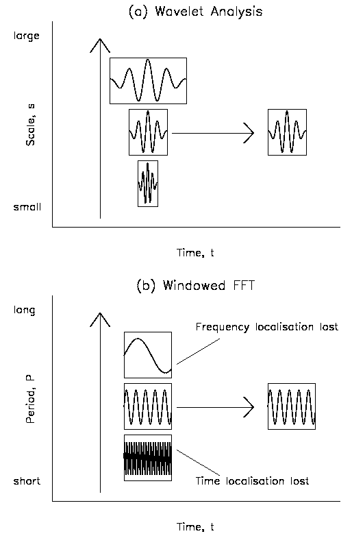
Like many time series in solar physics (and astronomy in general), light curves from NBPs are known to exhibit non-stationarity. This means that while the light curve may contain periodic signals, these may vary in both frequency and amplitude with time. As such, a simple Fourier analysis may not detect the time- and frequency-localised oscillations. There are several solutions to this problem. One such solution is to use a windowed FFT, whereby a portion of the light curve is selected, and this window is slid along the light curve, calculating the FFT at each step. However this approach means the shape of the curve is dependent on the window size. As is shown in Figure 5.3b, at low frequencies so few oscillations will occur inside the window that frequency-localisation will be lost. At high frequencies there will be so many oscillations inside the window that the time-localisation will be lost. The use of a box-car shape window will also lead to ringing effects.

Wavelet analysis circumvents these difficulties by using a base wave-packet of finite duration, d, and specific frequency, ν. A convolution of this wave-packet with a section of light curve will give an indication of the oscillatory power (at frequency ν) in that section (of duration d) of the light curve. Sliding this wave-packet along the light curve provides time-localisation. Changing the width of the wave-packet (known as the scale) provides frequency-localisation. The major improvements of wavelet analysis over a windowed FFT are,
(i) wavelet analysis will fit the same number of oscillations for each frequency whereas the windowed FFT does not (Figure 5.3).
(ii) a suitable choice of base-wavelet avoids edge effects.

Figure 5.4: The real part (blue) of the Morlet wavelet is simply a sine curve (green), with a Gaussian envelope (red)

In this work a wavelet analysis (Torrence & Compo 1998) was carried out on all the maximum threshold light curves using a Morlet wavelet of the form

where η = t/s is the dimensionless time parameter, t is the time, s the scale of the wavelet (i.e., its duration), ω₀ = sω is the dimensionless frequency parameter (i.e., the number of oscillations within the wavelet; ω₀=6 to satisfy the admissibility condition, Farge 1992), and π^-1/4 is a normalization term. The real part of this wavelet is basically a sine curve, with a Gaussian envelope (Figure 5.4). This continuous (and hence nonorthogonal), complex function is ideal for capturing smooth, continuous oscillatory behaviour, but is known to be redundant at large scales (and hence low frequencies) where the wavelet spectrum will be highly correlated (another reason for filtering off low frequencies). The wavelet transform, W_n, at scale, s, of a discrete sequence, x_n (n=0, 1, 2, .... N-1) is a convolution of x_n with a translated Ψ(η)

The smallest scale, s₀ is normally chosen as 2δt (i.e., inverse of the Nyquist frequency) with the larger scales then 2ⁿ multiples of s₀,

where δj is the spacing between scales and j=0, 1, 2... J-1. Hence the scales values increase logarithmically from s₀ to s₀ x 2^Jδj and J is calculated by rearranging Equation 81,

The wavelet transform will have a real and imaginary part, from which the amplitude, power, and phase can be determined as for the FFT. These will all be 2-dimensional maps, plotted against both time and scale (here scale, period, and frequency can be interchanged). Significance levels can also be calculated using a method similar to that for the FFT (e.g., for sig = 0.95, χ² (0.05,2) = 5.99, which is then multiplied by the mean power spectrum to give a power value for the 95% level).

Bocchialini & Baudin (1995) note that although wavelet analysis can be used to obtain phase information, this is very sensitive to frequency. They preferred to determine lags from correlations between their signals, and it is an extension of their method which is used here. Essentially, from the 2D wavelet power density maps, `power curves' at each frequency were created by taking slices of the wavelet power transform. These were then cross correlated across pairs of wavelengths to search for timelags (it should also be noted here that the chosen width of the frequency band should be small enough to negate errors arising from the different weighting of each scale, Torrence & Compo 1998).