Contrast Lightcurves

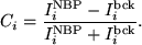
Lightcurves were created using the following method. For a single image i, a histogram of the pixel intensity is constructed, from which I^Mod, the most common (modal) pixel value of the image, is selected to represent the background. A threshold pixel intensity, I^thr is then chosen to contour the NBP. All pixels inside this contour are included in the NBP, and I^NBP is calculated as the average intensity value of all these pixels. A further improvement on previous work is achieved by not choosing a constant absolute threshold for each image in the series. Instead a constant relative threshold is chosen throughout, as a number of standard deviations above the mean for the (invariably different) standard deviation and mean of each image. The contrast, C_i, of each image, i, is then defined as,

This is repeated for every image in the sequence for a given threshold, such that the final lightcurve is then a series of C_i values.

Figure 4.2: Choice of threshold for an NBP. Top row (Image A) - Left plot: Histogram of pixel intensities. The solid line is at the mean, and the dashed line is at 2σ above the mean. Right image: The dashed contour is at the intensity value given by the dashed line of the plot on the left. Bottom row (Image B) - Left plot: Histogram of pixel intensities resulting from the same image as the top row, but with 10% less intensity. The solid line is at the mean, the dashed line is at 2σ above the mean, and the dash-dot line is at the same absolute threshold as the top row. Right image: Both the dashed and dash-dot lines are contoured at the intensities given by the plot on the left. The dash contour on the bottom image contains the same pixels as the contour on top image. The dash-dot contour contains fewer pixels.

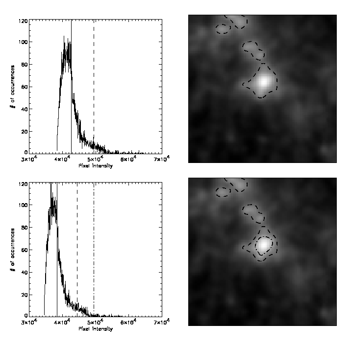This lightcurve construction removes any long-term trend due to sky fluctuations. For example, assume an NBP exhibits no change in intensity but a thin cloud results in a decreased intensity of 10% between two sequential images, A & B (Figure 4.2). Hence I^Mod, the mean (), and the standard deviation (σ) will all decrease by 10% in the second image. If the same absolute threshold intensity is used in both images, fewer pixels will be contoured in image B (Figure 4.2 dash-dot line), which will alter I^NBP erroneously. However if a constant relative threshold (e.g., 2σ above the mean) is used, the same exact pixels will be contoured in each image (Figure 4.2 dash line). As this results in a decrease of 10% in both I^Mod and I^NBP the contrast value of each image will be the same.

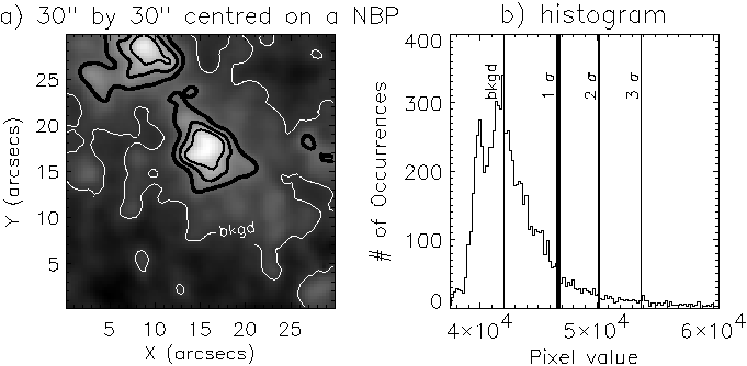
Figure 4.3: Description of thresholding contours on an NBP. (a) Sample NBP. The dark lines show the contour for all pixels in the image which are 1.0σ (thickest line), 2.0σ, and 3.0σ (thinnest line) above the mean. Only pixels inside the three centre-most contours are included. The white line contours the background level.(b) Corresponding histogram of the sample image. The background level is the modal value. The three vertical lines refer to the contour levels of (a).

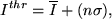
After the creation of the contrast lightcurve the threshold value was increased and a new lightcurve created. The threshold was chosen to increase from a minimum of above the mean, in steps of 0.05σ

n ∈ (1.0, 1.05, 1.10, .... N), where N is chosen so that the contour confines at least ten pixels in all images in the sequence (this normally occurred in only one image per sequence, such that the average number of pixels in an image at maximum threshold was around one hundred). With this method, increasing the threshold corresponds to better isolation of the very centre of the NBP (Figure 4.3a), and provides a means of probing and comparing different parts of the NBP. Essentially this increasing threshold creates a series of nested contours in the NBP.

This `contour & contrast' method can only be applied to data with a high spatial resolution in two simultaneous spatial dimensions and with good seeing conditions. A low spatial resolution means few pixels will be contoured at high threshold. Spectrometers normally only have one spatial dimension so require an image to be built up by scanning the slit across a region. The final image will therefore contain contributions from different points in time. In 'sit and stare' mode the slit may be too small to contour the NBP correctly, and causes an extra low-frequency cutoff (Section 4.1). Finally, poor seeing will lead to poor image contrast, increasing the difficulty of separating the NBP from the background intensity.