Given a set of observations/data, one often wants to summarize and get at underlying physics by fitting some sort of model to the data. The model might be an empirical model or it might be motivated by some underlying theory. In many cases, the model is parametric: there is some number of parameters that specify a particular model out of a given class.
The general scheme for doing this is to define some merit function that is used to determine the quality of a particular model fit, and choose the parameters that provide the best match, e.g. a minimum deviation between model and data, or a maximum probability that a given set of parameters matches the data.
When doing this one also wants to understand something about how reliable the derived parameters are, and also about how good the model fit actually is, i.e. to what extent it is consistent with your understanding of uncertainties on the data.
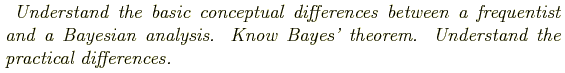
There are two different ``schools" about how to think about model fitting: frequentism and Bayesian. In the frequentist approach (sometimes called the classical approach), one considers how frequently one might expect to observe a given data set given some underlying model (i.e., P(D| M), the probability of observing a data set given a model); if very infrequently, then the model is rejected. The model that produces the observed data most frequently is viewed as the correct underlying model, and as such, gives the best parameters, along with some estimate of their uncertainty.
The Bayesian approach considers the probability that a given model is correct given a set of data (i.e. P(M| D), the probability of a model given a dataset). It allows for the possibility that there is external information that may prefer one model over another, and this in incorporated into the analysis as a prior. It considers the probability of different models, so talks about probability distribution functions of parameters. Examples of priors: fitting a Hess diagram with a combination of SSPs, with external constraints on allowed ages; fitting UTR data for low count rates in the presence of readout noise.
The frequentist paradigm has been mostly used in astronomy up until fairly recently, but the Bayesian paradigm has become increasingly widespread. In many cases, they can give the same result, but with somewhat different interpretation, but in some cases, results can differ. The basic underpinning of Bayesian analysis comes from Bayes theorem of probabilities:
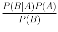
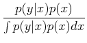
where P(A| B) is the conditional probability, i.e. the probability of A given that B has occurred. This can be understood fairly easily. Imagine there is some joint probability distribution function of two variables, p(x, y) (see ML 3.2; imagine, for example, that this could be distribution of stars as a function of effective temperature and luminosity!). Then, thinking about slices in each direction to get to the probability at a given point, we have:
This gives:

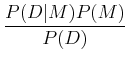
In the context of Bayesian analysis, we can talk about the probility of models, and we have:
In practice, frequentist analysis yields paramters and their uncertainties, while Bayesian analysis yields probabilitiy distribution functions of parameters. The latter is often more computational intensive to calculate. Bayesian analysis includes explicit priors.
For some more detailed discussion, see http://arxiv.org/abs/1411.5018
Let's start with a frequestist analysis, because in many cases, this provides a component of the Bayesian analysis. Given a set of data and some model (with parameters), one considers the probability that the set of data will be observed if the model is correct, and we will prefer the set of parameters that maximizes this probability.
Consider the example of fitting a straight line to a set of data. How is the best fit line usually determined? (least squares).
Where does this come from? Consider that observed data points have some
measurement uncertainty, ![]() . For now consider that all points have
the same uncertainty, i.e. homoschedastic uncertainties, and that
the uncertainties are distributed according to a Gaussian distribution.
. For now consider that all points have
the same uncertainty, i.e. homoschedastic uncertainties, and that
the uncertainties are distributed according to a Gaussian distribution.
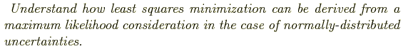
What is the probability of observing a given data value from a known Gaussian distribution? What's the probability of observing a series of two independently drawn data values?
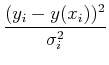
The probability of observing a series of data points is, given some model y(xi| aj):
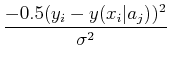
Maximizing the probability is the same thing as maximizing the logarithm of the probability, which is the same thing as minimizing the negative of the logarithm, i.e. minimize:
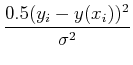
If ![]() is the same for all points, then this is equivalent to minimizing
is the same for all points, then this is equivalent to minimizing
Consider a simple application, multiple measurements
of some quantity, so the model is
y(xi) = ![]() where we want to
determine the most probable value of the quantity, i.e.
where we want to
determine the most probable value of the quantity, i.e. ![]() . What's
the answer?
. What's
the answer?
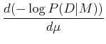
Minimizing gives:
 = 2
= 2What about the case of unequal uncertainties on the data points, i.e. heteroschedastic uncertainties? Then
Often, people qualititatively judge the quality of a fit by the
reduced ![]() , or
, or ![]() per degree of freedom:
per degree of freedom:

It is important to recognize that this analysis depends on the assumption that the uncertainties are distributed according to a normal (Gaussian) distribution!
Using ![]() as a method for checking uncertainties, or even determining
them (at the expense of being able to say whether your model is
a good representation of the data!). See ML 4.1
as a method for checking uncertainties, or even determining
them (at the expense of being able to say whether your model is
a good representation of the data!). See ML 4.1

For our simple model of measuring a single quantity, we have:
= 2 = 0
= 0

Let's apply this to a slightly more complicated example: fitting a straight line to a set of data. Here, the model is
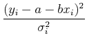
Again, we want to minimize ![]() , so we take the derivatives with
respect to each of the parameters and set them to zero:
, so we take the derivatives with
respect to each of the parameters and set them to zero:
Separating out the sums, we have:
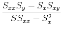
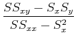
![]()
We also want the uncertainties in the parameters. Again, use propagation of errors to get (work not shown!):


Finally, we will want to calculate the probability of getting ![]() for our fit, in an effort to understand 1) if our uncertainties are not
properly calculated and normally distributed, or 2) if our model is a
poor model.
for our fit, in an effort to understand 1) if our uncertainties are not
properly calculated and normally distributed, or 2) if our model is a
poor model.
Let's do it. Simulate a data set, fit a line, and output parameters, parameter uncertainties, chi2, and probability of chi2.
We can generalize the least squares idea to any model that is some linear combination of terms that are a function of the independent variable, e.g.
such a model is called a linear model, because it is linear in the parameters (but not at all necessarily linear in the independent variable!). The model could be a polynomial of arbitrary order, but could also include trignometric functions, etc. We write the model in a simple form:
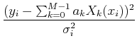
where there are M parameters. We will still have N data points and, as you might imagine, we require N > M. We can write the chi-squared merit function as:
Then, minimizing ![]() leads to the set of M equations:
leads to the set of M equations:
Separating the terms and interchanging the order of the sums, we get:
 =
= 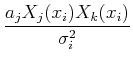
Define:


Sometimes these equations are cast in terms of the design matrix, A, which consists of N measurements of M terms:

For a given data set, we can calculate ![]() and
and ![]() either by
doing the sums or by setting up the design matrix and using matrix
arithmetic. We then need to solve the set of equations for ak.
either by
doing the sums or by setting up the design matrix and using matrix
arithmetic. We then need to solve the set of equations for ak.
Note that this formulation applies to problems with multiple independent variables, e.g., fitting a surface to a set of points; simply treat x as a vector of data, and the formulation is exactly the same.
This is just a linear algebra problem, and there are well-developed
techniques (see Numerical Recipes chapter 2). Most simply, we just
invert the matrix ![]() to get
to get
A simple algorithm for inverting a matrix is called Gauss-Jordan elimination, and there are others. In particular, NR recommends the use of singular value decomposition for solving all but the simplest least-squares problems; this is especially important if your problem is nearly singular, i.e. where two or more of the equations may not be totally independent of each other: fully singular problems should be recognized and redefined, but it is possible to have non-singular problems encounter singularity under some conditions depending on how the data are sampled. See NR 15.4.2 and Chapter 2!
As an aside, note that it is possible to solve a linear set of equations
significantly faster than inverting the matrix through various types of
matrix decomposition, e.g., LU decomposition and Cholesky decomposition
(again, see NR Chapter 2). There may be linear algebra problems that
you encounter that only require the solution of the equations and not
the inverse matrix. However, for the least squares problem, we often
actually do want the inverse matrix
C = ![]() , because its elements
have meaning. Propagation of errors gives:
, because its elements
have meaning. Propagation of errors gives:
A Python implementation of matrix inversion and linear algebra in general can be found in scipy.linalg, e.g., and here is the summed matrix implementation for a straight line fit (but the functional form only comes in through the derivative function!):
def deriv(x) :
    # if x is numpy array, then we can return vectors of derivatives
    try :
        return [np.ones(len(x)),x]
    except :
        return [1.,x]

# data points in (x,y)
# loop over parameters, sums over data points (y) are done with vector arithmetic
for k in np.arange(npar) :
    beta[k] = np.sum(deriv(x)[k]*y/sigma**2)
    for j in np.arange(npar) :
        alpha[k,j] = np.sum(deriv(x)[k]*deriv(x)[j]/sigma**2)
c=np.linalg.inv(alpha)
print np.dot(c,beta)
Here is the design matrix approach to the sums:
A = np.vander(x, 2)  # Take a look at the documentation to see what this function does!
ATA = np.dot(A.T, A / yerr[:, None]**2)
w = np.linalg.solve(ATA, np.dot(A.T, y / yerr**2))
V = np.linalg.inv(ATA)
Linear least squares is also implemented in astropy in the modeling module using the LinearLSQFitter class (which uses numpy.linalg); astropy has a number of standard models that you might use, or you can provide your own custom model.
from astropy.modeling import models, fitting
fit_p = fitting.LinearLSQLSQFitter()
p_init = models.Polynomial1D(degree=degree)
pfit = fit_p(p_init, x, data)
Astropy has a number of common models, but you can also define your own model using models.custom_model, by supplying a function that returns values, and a function that returns derivatives with respect to the parameters.

Note that for problems with large numbers of parameters, the linear algebra can become very computationally expensive. In many cases, however, the matrix that represents these problems may only be sparsely populated, i.e. so-called sparse matrices (see Numerical Recipes 2.7, Figure 2.7.1).
Example: spectral extraction
In such cases, there are methods that allow the equations to be solved significantly more efficiently.
However, not all fits are linear in the parameters .... which of the following are not?
In a linear fit, the ![]() surface is parabolic in parameter space,
with a single minimum, and linear least squares can be used to determine
the location of the minimum. In the non-linear case, however, the
surface is parabolic in parameter space,
with a single minimum, and linear least squares can be used to determine
the location of the minimum. In the non-linear case, however, the
![]() surface can be considerably more complex, and there is a (good)
possibility that there are multiple minima, so one needs to be concerned
about finding the global minimum and not just a local minimum. Because
of the complexity of the surface, the best fit is found by an iterative
approach.
surface can be considerably more complex, and there is a (good)
possibility that there are multiple minima, so one needs to be concerned
about finding the global minimum and not just a local minimum. Because
of the complexity of the surface, the best fit is found by an iterative
approach.
A conceptually simple approach would be a grid search, where one simply
tries all combinations of parameters and finds the one with the lowest ![]() .
Obviously, this is extremely computationally inefficient, especially for problems
with more than a few parameters! One is also forced to decide on a step size in the
grid, although you might imagine a successively refined grid as you proceed.
But in general, this method is not recommended, apart from occaisionally trying
it to try to ensure that your more efficient solution is not landing in a local
minimum.
.
Obviously, this is extremely computationally inefficient, especially for problems
with more than a few parameters! One is also forced to decide on a step size in the
grid, although you might imagine a successively refined grid as you proceed.
But in general, this method is not recommended, apart from occaisionally trying
it to try to ensure that your more efficient solution is not landing in a local
minimum.
Better approaches attempt to use the ![]() values to find the minimum more
efficiently. They can generally be split into two classes: those that use the
derivative of the function and those that don't. If you can calculate derivatives
of
values to find the minimum more
efficiently. They can generally be split into two classes: those that use the
derivative of the function and those that don't. If you can calculate derivatives
of ![]() with respect to your parameters, then this provides information about
how far you can move in parameter space towards the minimum. If you can't calculate
derivates, you can evaluate
with respect to your parameters, then this provides information about
how far you can move in parameter space towards the minimum. If you can't calculate
derivates, you can evaluate ![]() at several different locations, and use
these values to try to work your way towards the minimum.
at several different locations, and use
these values to try to work your way towards the minimum.
With derivatives, the approach has a fairly close parallel to the linear
least squares problem. Around the final minimum, the ![]() surface can
be approximated as a parabola, and it is possible to correct the solution to
the minimum solution if one can arrive at a set of parameters near to the
final minimum. This is acheived via the set of equations:
surface can
be approximated as a parabola, and it is possible to correct the solution to
the minimum solution if one can arrive at a set of parameters near to the
final minimum. This is acheived via the set of equations:
where

 =
= 
 - (yi - y(xi| a))
The matrix
![]() is known as the curvature matrix. In most cases, it seems to be
advisable to drop the second derivative term in this matrix, see NR 15.5.1 for a
partial explanation, so the standard approach uses:
is known as the curvature matrix. In most cases, it seems to be
advisable to drop the second derivative term in this matrix, see NR 15.5.1 for a
partial explanation, so the standard approach uses:
To implement this, you choose a starting guess of parameters, solve for the corrections
![]() al to be applied
to a current set of parameters, and iterates until one arrives at a solution that does not change significantly.
al to be applied
to a current set of parameters, and iterates until one arrives at a solution that does not change significantly.
Far from the solution, this method can be significantly off in providing a good correction, and, in fact, can
even move parameters away from the correct solution. In this
case, it may be advisable to simply head in the the steepest downhill direction in ![]() space, which
is known as the method of steepest descent. Note that while this sounds like a reasonable thing
to do in all cases, it can be very inefficient in finding the final solution (see, e.g.
NR Figure 10.8.1).
space, which
is known as the method of steepest descent. Note that while this sounds like a reasonable thing
to do in all cases, it can be very inefficient in finding the final solution (see, e.g.
NR Figure 10.8.1).
A common algorithm switches between the method of steepest descent and the parabolic approximation and is known as the Levenberg-Marquardt method. This is done by using a modified curvature matrix:
where
When ![]() is large, this gives a steepest descent method, when small, a parabolic method. This
leads to the following recipe:
is large, this gives a steepest descent method, when small, a parabolic method. This
leads to the following recipe:
Two key issues in nonlinear least squares is finding a good starting guess and a good convergence
criterion. You may want to consider multiple starting guesses to verify that you're not converging
to a local minimum. For convergence, you can look at the amplitude of the change in parameters or
the amplitude in the change of ![]() .
.
This method in implemented in astropy in the modeling module using the LevMarLSQFitter which is used identically to the linear least squares fitter described above.
There are certainly other approaches to non-linear least squares, but this provides an introduction.
A common minimization method that does not use derivatives is the ``downhill simple" or Nelder-Mead algorithm.
For this technique, ![]() is initially evaluated at M + 1 points (where M is the number of paramters).
This makes an M-dimensional figure, called a simplex. The largest value
is found, and a trial evalaution is made at a value reflected through the
volume of the simplex. If this is smaller than the next-highest value of
the original simplex, a value twice the distance is chosen and tested;
if not, then a value half the distance is tested, until a better value is
found. This point replaces the initial point, and the simplex has moved
a step; if a better value can't be found, the entire simplex is contracted
around the best point, and the process tries again.
The process in then repeated until a convergence criterion is
met. See NR Figure 10.5.1
and section 10.5. The simplex works its way
down the
is initially evaluated at M + 1 points (where M is the number of paramters).
This makes an M-dimensional figure, called a simplex. The largest value
is found, and a trial evalaution is made at a value reflected through the
volume of the simplex. If this is smaller than the next-highest value of
the original simplex, a value twice the distance is chosen and tested;
if not, then a value half the distance is tested, until a better value is
found. This point replaces the initial point, and the simplex has moved
a step; if a better value can't be found, the entire simplex is contracted
around the best point, and the process tries again.
The process in then repeated until a convergence criterion is
met. See NR Figure 10.5.1
and section 10.5. The simplex works its way
down the ![]() surface, expanding when it can take larger steps,
and contracting when it needs to take smaller steps. Because of this
behavior, it is also known as the ``amoeba" algorithm.
surface, expanding when it can take larger steps,
and contracting when it needs to take smaller steps. Because of this
behavior, it is also known as the ``amoeba" algorithm.
Python/scipy implementation of Nelder-Mead
Python/scipy summary of optimization routines in general
Fitting provides us a set of best-fit parameters, but, because of uncertainties and limited number of data points, these will not necessarily be the true parameters. One generally wants to understand how different the derived parameters might be from the true ones.
The covariance matrix gives information about the uncertainties on the derived parameters. In the case of well-understood uncertainties that are strictly distributed according to a Gaussian distribution, these can be used to provide confidence levels on your parameters; see NR 15.6.5.
In some cases, however, you may not be in that situation. Given this, it is common to derive parameter uncertainties by numerical techniques.
A straightforward technique if you have a good understanding of your measurement uncertainties is Monte Carlo simulation. In this case, you simulate your data set multiple times, derive parameters for each simulated data set, and look at the range of fit parameters as compared with the input parameters. To be completely representative of your uncertainties, you would need to draw the simulated data set from the true distribution, but of course you don't know what that is (it's what you're trying to derive)! So we take the best-fit from the actual data as representative of the true distribution, and hope that the difference between the derived parameters from the simulated sets and the input parameters is representative of the difference between the actual data set and the true parameters.
If you don't have a solid understanding of your data uncertainties, then Monte Carlo will not give an accurate representation of your parameter uncertainties. In this case, you can use multiple samples of your own data to get some estimate of the parameter uncertainties. A common technique is the bootstrap technique, where, if you have N data points, you make multiple simulations using the same data, drawing N data points from the original data set - with replacement (i.e. same data point can be drawn more than once), derive parameters from multiple simulations, and look at the distribution of these parameters.
However, you may need to be careful about the interpretation of the confidence intervals determined by any of these techniques, which are based on a frequentist interpretation of the data. For these calculations, note that confidence intervals will change for different data sets. The frequentist interpretation is that the true value of the parameter will fall within the confidence levels at the frequency specified by your confidence interval. If you happen to have taken an unusual (infrequent) data set, the true parameters may not fall within the confidence levels derived from this data set!
Review material above, also see astroML, NR and http://arxiv.org/abs/1411.5018
As discussed above and in additional references, Bayesian analysis has several significant differences from the frequentist/likelihood approach. First, Bayesian analysis calculates the probability of model parameters given data, rather than the probability of data given a model.
Practically, this allows for the possibility of specifying an explicit prior on the model parameters. The Bayesian analysis may give the same result as the frequentist analysis for some choices of the prior, but it makes the prior explicit, rather than hidden.
Second, the Bayesian analysis produces a joint probability distribution function of the model parameters. The frequentist analysis produces a most probable set of parameters and a set of confidence intervals.
The Bayesian analysis is computationally more challenging because you actually have to compute the probability for different model parameters. This is essentially performing a grid search of the full parameter space, which can be computationally intractable for large numbers of parameters. Fortunately, computational techniques have been developed to search through the full parameter space concentrating only on the regions with non-negligible probability; as discussed below, Markov Chain Monte Carlo is foremost among such techniques.
Priors in Bayesian analysis reflect external knowledge about parameters that exist independent of the data being analyzed. If there is no external knowledge, then you want to use a noninformative prior. Often, this is just a statement that all parameter values are equally likely. In many cases, this makes a Bayesian analysis equivalent to a frequentist analysis. However, beware that model parameters could be expressed with a transformation of variables, and a flat distribution in one variable may not be a flat distribution under a variable transformation, and could lead to different results. Also, a prior that appears to be unbiased may not be so, e.g., consider the fitting parameters for a straight line, in particular the slope.
Lots of literature on the subject.
For many problems, only some of the parameters are of interest, while others fall into the category of so-called nuisance parameters, which may be important for specifying an accurate model (which is fundamentally important!), even though they may not be of interest for the scientific question you are trying to answer. In such cases, Bayesian analysis uses the concept of marginalization, where one integrates over the dimensions of the nuisance parameters to provide probability distribution functions of only the parameter(s) of interest.
Marginalization is also used to give probability distribution functions of individual parameters, i.e. without regard to the values of other parameters. However, one needs to beware that parameter values may be correlated with each other, and marginalization hides such correlations.
Marginalization can also be used to derive the probability distribution of some desired quantity given measurements of other quantities if there is some relation between the measured and desired quantity. An example is in determining ages of stars given a set of observations, e.g. of spectroscopic parameters and/or apparent magnitudes. Here, stellar evolution gives predictions for observed quantities as a function of age, mass, and metallicity; in conjunction with an initial mass function, you get predictions for number of stars for each set of parameters. Given some priors on age, mass, and/or metallicity, you could compute the probability distribution of a given quantity by marginalizing over all other parameters. Observational constraints would modify this probability distribution.
![]()
Calculating marginal probability distributions is basically a big integration problem. If the problem has many parameters, the multi-dimensional integral can be very intenstive to calculate. One technique for multi-dimensional integration is Monte Carlo integration. Here, you just choose a (large) number of points at random within some specified volume (limits in multiple dimensions), sample the value of your function at these points and estimate the integral as:
We could use this to calculate marginal probability distribution functions, but it is likely to be very inefficient if the probability is small over most of the volume being integrated over. Also, for most Bayesian problems, we do not have a proper probability density function because of an unknown normalizing constant; all we have is the relative probability at differet points in parameter space.
To overcome these problems, we would instead like to place points in a volume proportional to the probability distribution at that point; we can then calculate the integral by summing up the number of points. This is achieved by a Markov Chain Monte Carlo analysis. Here, unlike Monte Carlo, the points we choose are not statistically independent, but are chosen such that the sample the (unnormallized) probability distribution function in proportion to its value. This is achieved by setting up a Markov Chain, which means a process where the value of a sampled point depends only on the value of the previous point. To get the Markov Chain to sample the (unnormalized) PDF, the transition probability has to satisfy:
Now, to do the integral, we just sum the number of points in the chain at the different parameter values.
There are multiple schemes to generate such a transition probability. A common one is called the Metropolis-Hastings algorithm. In this algorithm, from a given point, generate a candidate step from some proposal distribution, q(x2| x1),that is broad enough to move around in the probability distribution q(x2| x1) is steps that are not too large or too small. If the candidate step falls at a larger value of the probability function, accept it, and start again. If it falls at a smaller value, accept it with probability proportional to
For a symmetric Gaussian proposal definition, note that the q values cancel out.
Note that you need to choose a starting point. If this is far from the maximum of the probability distribution, it may take some time to get to the equilibrium distribution. This leads to the requirement of a burn-in period for MCMC algorithms.
So, in practice, you have to be careful about choosing an appropriate proposal distribution, and an appropriate burn-in period.
Implementation: see emcee and pymc, among others, also , here
Note that emcee uses an algorithm that is different from Metropolis-Hastings, that is designed to function more efficiently in a case where the PDF may be very narrow, leading to very low acceptance probabilities with Metropolic-Hastings. Partly this is accomplished by using a number of walkers, i.e. multiple different Markov chains, but these are not totally independent: knowledge from other walkers are used (somehow) to help explore the parameter space more efficiently. Note that since the walkers are not independent, the chain from a single walker does not sample the PDF proportionally; the combined chain from all of the walkers is what needs to be used.