Algorithms

Writing a program

Some simple suggestions on developing a program/algorithm:

1. Think about what you want to do! make sure you fully understand the question/problem before starting to write code. Outline the methdology you will use in words, diagrams or figures, so you make sure you understand what you want to do before you get caught up in syntax, etc. problems
2. Start to generate the code. If possible, do it in pieces, and check each piece one at a time. Include comments in what you do, which serve not only as documentation, but keep you on track with your plan. Include some debugging statements, considering the possibility of building in a ``verbosity" level from the start. Consider building in error trapping from the star
3. Once it seems to be working, test your code. Try to think of using it in an unexpected way to see what happens. Do you best to find what is wrong with it, not what is right.
4. Go back through your code and see if you can clean it up in any way Is there repeated code that can be consolidated? Are there more efficient or transparent ways to write things?
5. Make sure your code is fully commented. Again, this doesn't mean write a comment for every line! You want to keep the code readable, with comments used to document the overall strategy and points of the code that are not immediately understandable from the code itself.

Speed and scaling

Lists and list matching

(sorting, finding items, matching lists, etc.)

Random number generation

(see Numerical Recipes Chapter 7)

Many situations in analysis lead you to want to provide a ``random" distrbution of numbers. High among these are simulating data sets to test analysis routines. Random numbers also play a significant role in numerical simulations.

Considerable literature on the subject, and significant improvements of the past several decades. Be aware that lousy random number generators exist! So if it is important, research your random number generator. See, e.g., diehard tests.

Computer generated random numbers are repeatable! Generally start with a seed number; many random number generators will use clock time if seed isn't specified. Users are strongly encouraged to record their seed(s) in case repeatability is desired (e.g, say you make some modification to your code, but want to make sure you can still repeat past results under the same conditions).

Lowest level random number generators give uniform deviates, i.e., equal probability of results in some range (usually 0 to 1 for floats). E.g., python random.random, random.seed, numpy.random.random , numpy.random.seed

Exercise: generate sets of increasing larger uniform deviates, plot histograms.

What if you want random number for some other distributions? e.g., Gaussian, Poisson, luminosity function, mass function ...

Transformation method: consider cumulative distribution of desired function. This is a function that varies between 0 and 1. Choose a uniform random deviate between 0 and 1, and look up what value of the cumulative distribution this corresponds to, and you have your deviate in your function! This does require that you can integrate your function, and then invert that integral.

Figure NR 7.3.1 See NR 7.3.1 in-class exercise: generate random deviates for a ``triangular" distribution: p(x) $\propto$ x. What is constant of proportionality to make probability distribution? Use the relation to generate random deviates, and plot them with a histogram.

y = 2x

F = $$\int$$ydx = x²

x(F) = $$\sqrt{(}$$F)

What if you can't integrate and invert your function? Rejection method: choose a function that you can integrate and invert that is always higher than your desired distribution. Choose a random deviate as before and look up corresponding value in the comparison function. Calculate value of both desired function and comparison function. Choose a uniform deviate between 0 and c(x): if it is larger than f(x), reject your value and start again! So requires 2 random deviates for each attempt, and the number of attempts before you get a deviate in your desired distribution depends on how close your comparison function is to your desired function.

Figure NR 7.3.2 See NR 7.3.2 Example demonstration: truncated Gaussian distribution. Generate random deviates with rejection method.

Lots of other clever ways to generate deviates in desired functions, see Numerical Recipes, chapter 7

Common distributions: Gaussian, Poisson:

P(x,$$\mu$$,$$\sigma$$) = $${1 \over \sqrt{2\pi} \sigma}$$e^{${-{(x-\mu)^2\over 2\sigma^2}}$}

P(x,$$\mu$$) = $${\mu^x \exp^{-\mu} \over x!}$$

typical situations in which these apply. Poisson: counting statistics, Gaussian: distribution of many physical quantities, reasonable approximation to Gaussian for large mean. For these common distributions, accurate and fast ways of generating random deviates have been developed.

Python implementations: numpy.random.normal, numpy.random.poisson

in class exercise: simulate some data, e.g. a linear relation (x=1,10, y=x) with Gaussian (mean=0, sigma=various) scatter. Plot it up.

alternate: CMD from isochrones with Poisson scatter in colors and magnitudes.

Interpolation

(see Numerical Recipes Chapter 3)

There are many situations in which you might have a tabulated or measured set of data, and want to get the values at intermediate locations in your data set, i.e. interpolation; for example, inverting a function (e.g., random deviates as above, wavelength calibration, etc.), resampling data (images or spectra), etc.

A key overall point about interpolation: when you interpolate, you are making some assumptions about the underlying nature of your data! Your result is only as good as your assumptions, and one can certainly imagine pathological cases!

Simplest interpolation: linear interpolation. Value at some intermediate location, x, between two points, x_i and x_i+1:

f (x) = Ay_i + By_i+1

A = $${(x_{i+1} - x)\over (x_{i+1}-x_i)}$$

B = $${(x - x_i)\over (x_{i+1}-x_i)}$$

Polynomial interpolation: Lagrange formula gives value polynomial of degree k going through k+1 points at arbitrary position, x, as a function of the tabulated data values:

L(x) = $$\sum_{{j=0}}^{k}$$y_jl_j(x)

l_j(x) = $$\prod_{{0\le m\le k,m\ne j}}^{}$$$${(x-x_m)\over(x_j-x_m)}$$

(note that this provides the values of the interpolating polynomial at any location without providing the coefficients of the polynomial itself). The coefficients are determined such that the polynomial fit goes exactly through the tabulated data points.

Beware, however, of thinking that higher order is necessarily better! Classic example:

f (x) = $${1.\over (1+25 x^2)}$$

Demonstrate interpolation for various npts, order. Note issues with even orders because this leads to using more tabulated points on one side of the desired value than the other (since even order means odd number of data points). At high order, polynomial can go wildly off, especially near data edges.

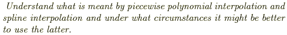
Another problem with piecewise polynomial interpolation, even at low order: the input data values that are used to interpolate to a desired location change as you cross each data point. This leads to abrupt changes in derivatives (infinite second derivative) of the interpolated function. For some applications, this can cause problems, e.g., if you are trying to fit an observed data set to some tabulated series of models, if you use derivatives to get the best fit.

This issue can be overcome using spline interpolation, which gives interpolated values that go through the data points but also provides continuous second derivative. Doing so, however, requires the use of non-local interpolation, i.e. the interpolating function includes values from all tabulated data points. Generally, people use cubic fits to the second derivatives, leading to cubic spline interpolation. To do cubic spline interpolation, one needs to specify boundary conditions at the ends of the data range: usually, a natural spline is adopted, with zero second derivatives at the ends, but it is also possible to specify a pair of first derivatives at the ends.

Cubic splines are probably the most common form of interpolation .... which doesn't necessarily mean the best in all circumstances.

Python implementation: scipy.interpolate.interp1d calucates interpolating coefficients for linear and spline interpolation, and can then be called to interpolate to desired position(s):

from scipy import interpolate

intfunc = interpolate.interp1d(xdata,ydata,kind='linear'|'slinear'|'quadratic'|'cubic'|order)

intfunc(x)  #returns interpolated value(s) at x

Exercise:

1. Define some function, func(x)

   def func(x) :
    .... your function here ...
   

2. For some given domain, plot your function at high sampling, e.g.:

    
   # get a high sampled array of independent variable
   x=numpy.linspace(xmin,xmax,1000)
   # plot the relation as a smooth line
   plt.plot(x,func(c)
   

3. For some given domain, sample your function with N points (evenly spaced, or maybe random?), e.g.:

    
   numpy.linspace(xmin,xmax,npts) # provides npts xdata points in your your domain
   plt.plot,xdata,func(data),'o') # plot data points as points
   

4. Determine the interpolating polynomial for linear and cubic spline, and overplot the interpolated function

   from scipy import interpolate
   # get the interpolating function (you need to choose which type)
   intfunc = interpolate.interp1d(xdata,func(xdata),kind='linear'|'slinear'|'quadratic'|'cubic'|order)
   # plot interpolated data at high sampling
   plt.plot(x,intfunc(x))
   

Fourier analysis basics and sinc interpolation

(see Numerical Recipes Chapter 12)

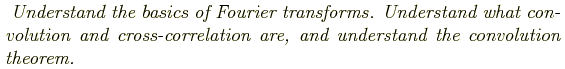
In many situations, it is useful to consider a series of data points using a Fourier decomposition; one application is a type of interpolation called sinc interpolation, but before we discuss that, a few Fourier basics. In Fourier analysis we can consider a function in two different representations: values in ``physical" space (e.g., time or location) vs. value ins ``frequency" space (e.g., temporal frequency or wavenumber). The two are related by Fourier transforms:

H(f )= $$\int$$h(x)exp$$\left(\vphantom{-2\pi i f x}\right.$$ -2$$\pi$$ifx$$\left.\vphantom{-2\pi i f x}\right)$$dx

h(x) = $$\int$$H(x)exp$$\left(\vphantom{2\pi i f x}\right.$$2$$\pi$$ifx$$\left.\vphantom{2\pi i f x}\right)$$df

(note that different implementations use different sign conventions, and sometimes people talk about angular frequency $\omega$ = 2$\pi$f.)

Physical interpretation is that a function can be decomposed into the sum of a series of sine waves, with different amplitudes and phases at each wavelength/frequency. Because we have amplitude and phase, the Fourier transform is, in general, a complex function.

Fourier transforms can be determined for discrete (as opposed to continuous) streams of data using the discrete Fourier transform, which replaces the integrals with sums. Algorithms have been developed to compute the discrete Fourier transform quickly by means of the Fast Fourier Transform (FFT); generally, this is done for data sets that are padded to a length of a power of 2. However, the FFT algorithm requires equally spaced data points. For unequally spaced points, one just has to do the full discrete Fourier transform.

Python implementations: numpy.fft, scipy.fftpack

import matplotlib.pyplot as plt
import numpy as np

# generate sine wave
x=np.linspace(0,10000.,8192)
y=np.sin(100*x)
plt.plot(x,y)

# fft
f=np.fft.fft(y)

# plot amplitude, try to get frequencies right....
plt.plot(np.abs(f))
plt.plot(np.fft.fftfreq(8192),np.abs(f))
plt.plot(np.fft.fftfreq(8192,100./8192),np.abs(f))

Two particular operations involing pairs of functions are of general interest: convolution and cross-correlation.

Convolution of two functions is defined as:

g(x)*h(x) = $$\int$$g(x')h(x - x')dx'

Usually, convolution is seen in the context of smoothing, where h(x) is a normalized function (with a sum of unity), centered on zero; convolution is the process of running this function across an input function to produce a smoothed version. Note that the process of convolution is computationally expensive; at each point in a data series, you have to loop over all of the points (or at least those that contribute to the convolution integrat). In some cases it can be advantageous to consider convolution in the Fourier domain, because of the convolution theorem, which states the convolving two functions in physical space is equivalent to multiplying the transforms of the functions in Fourier space. Multiplication of two functions is faster than convolution!

Python: numpy.convolve

Another useful function is the cross-correlation function:

g(x)$$\star$$h(x) = $$\int$$g(x')h(x' + x)dx'

which looks very similar to convolution (in fact, it is the same if h is a symmetric function), but is usually used quite differently. The cross-correlation is generally considered as a function of the lag, x; consider multiplying two functions and calculating the sum, then shifting one of the functions and doing it again, etc., and looking at the sums as a function of the shift. For two similar functions, the cross-correlation will be a maximum when the two functions ``line up", so this is useful for determining shifts between two functions (e.g., spatial shifts of images, or spectral shifts from velocity (but in velocity space, i.e. log(wavelength), not linear wavelength space). Cross-correlation can also be computed in the Fourier domain: it is equivalent to multiplying the Fourier transform of one function by the complex conjugate of the Fourier transform of the other. Note that the height and width of the cross-correlation function has information about the degree to which the two functions are similar.

A specific case of cross-correlation is the autocorrelation function, i.e., the cross-correlation of a function with itself.

OK, back to interpolation.

Sinc interpolation and the sampling theorem: see Bracewell chapter 10

When we sample a function at finite locations, we are multiplying by a sampling function, which is just a discrete set of impulses spaced by $\Delta$x. In the Fourier domain, this is convolving by the Fourier transform of the sampling function, which is a discrete set of frequencies spaced by 1/$\Delta$x.

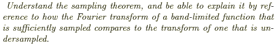
An important and useful result for interpolation is called the sampling theorem which arises in the case of a band-limited function, i.e. a function that has no power above some critical frequency. In this case, if one samples the function at sufficient frequency, which turns out to be twice the critical frequency, then it is possible to recover the entire function! Figure 10.3 from Bracewell shows the idea graphically. The critical frequency is known as the Nyquist frequency.

So all one does is Fourier transform the sampled function, multiply by a box function, and Fourier transform back. Alternatively, convolve the sampled function with the Fourier transform of a box function, which is the sinc function: sinc(x) = sin(x)/x. This leads to so-called sinc interpolation, which is the ideal interpolation in the case of a band-limited function.

Interpolation and uncertainties

Generally all interpolation schemes can be considered as a sum of data values multiplied by a set of interpolation coefficients at each point:

y(x) = $$\sum_{{i=0}}^{n}$$y_iP_i(x)

So far, we have been considering interpolation in perfect data. What if there are uncertainties on the data points? Clearly, these lead to uncertainties in the interpolated values. You can derive the uncertainties on these by error propagation, if the errors on the individual data points are uncorrelated:

$$\sigma$$(y(x))² = $$\sum$$$$\sigma$$(y(x_i))²P_i(x)²

However, now you have to be careful about how you use those errors, since the interpolated errors are now correlated, so using them properly requires you to use the full covariance matrix.

= $$\sigma_{u}^{2}$$$$\left(\vphantom{{{\partial{x}}\over{\partial {u}}}}\right.$$$${{\partial{x}}\over{\partial {u}}}$$$$\left.\vphantom{{{\partial{x}}\over{\partial {u}}}}\right)^{2}_{}$$ + $$\sigma_{v}^{2}$$$$\left(\vphantom{{{\partial{x}}\over{\partial {v}}}}\right.$$$${{\partial{x}}\over{\partial {v}}}$$$$\left.\vphantom{{{\partial{x}}\over{\partial {v}}}}\right)^{2}_{}$$ +2$$\sigma_{{uv}}^{2}$$$${{\partial{x}}\over{\partial {u}}}$$$${{\partial{x}}\over{\partial {v}}}$$

$$\sigma_{{uv}}^{2}$$ = lim(n - > $$\infty$$)$${1\over N}$$$$\sum$$(u_i - < u > )(v_i - < v > )

In the presence of noise (uncertainties), it is often advantageous to model the data by fitting an underlying function to a tabulated set of data points with some merit function criteria for determing what function provides the best fit. The fit can then be used to predict values at arbitrary location.

Beware of mixing and matching interpolation and fitting: doing fits on data sets with uncorrelated errors is substantially easier than doing them on data sets with correlated errors...

Differentiation and integration

Differentiation: finite differences

Integration: simple rules. extended rules. reaching a desired accuracy.

Monte Carlo integration

Differential equations

Runge-Kutta. Boundary value problems.