Single-Latitude Cut

This is the procedure for creating a single-latitude cut---one data cut with many "regions" taken at one latitude across many longitudes---with the IDL program CUTTER_GEN. The value of this method lies in obtaining a center-to-limb profile from several viewing geometries, thus providing better constraints on the model atmosphere. The problem is that this assumes one and the same cloud structure for all points in the data cut, which may be difficult to justify.

Two approaches used here reduce the likelihood of including significantly different cloud structures in a cut: (1) Only regions with similar spectra may be selected. (2) All regions are selected as close as possible to a single latitude.

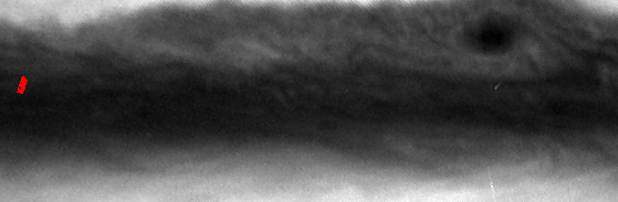
The following example of a data cut was not used in the modeling. The data cuts used can be viewed here.

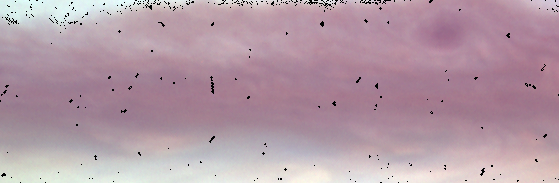
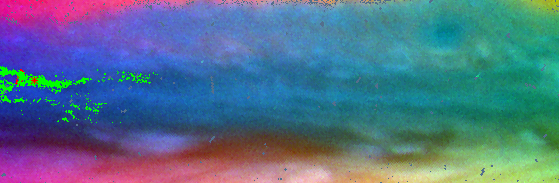
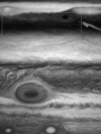
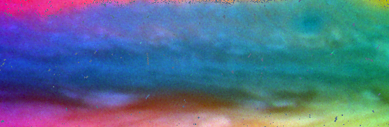
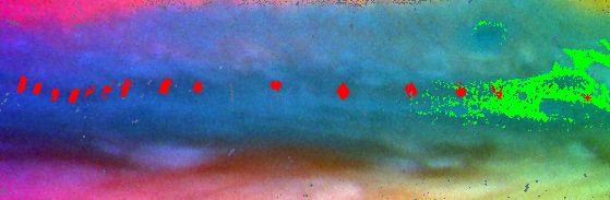
The user selects an area of the spectral image cube from the F410M image. PCA is then performed on this area. The false-color image (top right) shows the first 3 PCs (R=1st, G=2nd, B=3rd). (Gray pixels are masked due to cosmic rays or bad pixels.) A true-color image shows that a fairly uniform observed color (I/F spectra) is present running longitudinally across the North Equatorial Belt.

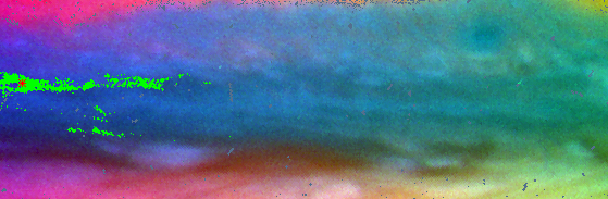
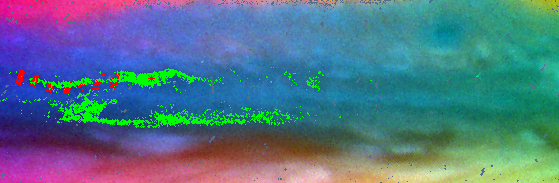
The user selects a fiducial point (red asterisk) from the PCA image to make a cut. Spectrally similar locations (green pixels) are found based on the PCA results (see SEL_PCA). The region added to the cut (red pixels) consists of locations that are both spectrally similar and within ± 0.0025 in μ and μ₀ for each image in the cube.

The individual regions of the data cut work like so: There are 11 images in this cube. In each image, the wavelength (λ), I/F, μ, μ₀, and phase angle (φ) are recorded for each pixel. One region has been created. All pixels within that region are averaged together. Thus, the data cut currently consists of 11 points in [λ, I/F, μ, μ₀, φ] space. When a second region is added, the pixels from that region will be averaged together---separately from the first region. Then the data cut will have 22 points in [λ, I/F, μ, μ₀, φ] space.

The user selects new fiducial points to add regions to the cut. Only those points that are spectrally similar to any previous fiducial point are allowed. The spectrally similar points associated with each fiducial point can be viewed here.

F255W

F343N

F375N

F390N

F410M

F437N

F469N

F502N

F673N

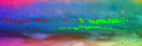
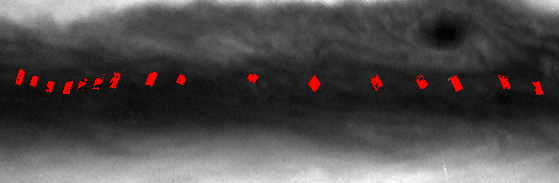
All desired regions are now selected (top). The subsequent images show the contrast in the selected data cut in each image of the cube. The dynamic range of the display is stretched to the minimum and maximum of the data cut in each image.

Note that in an ideal data cut: (1) No structure should be visible within each region. There should be no contrast at all, or there should only be noise. An example of a bad region is the last (far right) region in the F437N image. (2) Contrast between regions should vary smoothly with viewing angle. Note the nice center-to-limb variations in the two F673N images.

Go to the real data cuts and their SSA modeling results here.
Go to the PCA results for all data cuts here.