Kaggle Zillow Competition
This Kaggle Competition is being put on by Zillow, in an attempt to get users to improve their cost estimate by accurately modeling the logerror in their price estimates.
logerror = log( Zestimate ) - log( SalePrice )
This is a competition with over a million dollars in prize money, so while I don't expect to perform as well as a team gunning for the prize, I thought this would be a fun set to explore and see what I can do.
Zillow Data Exploration
Here I will include some highlights of my simple data exploration from the raw dataset. I will start by only using exploring data in the set from homes that have been sold:
The data set as of August 24th, 2017 contains over three million rows (or postings), and 60 columns of variables, two of which are our target logerror, and the transaction date. Only about 90k of these rows actually contain transactions, and we will focus this exploration on those with transactions for the time being.
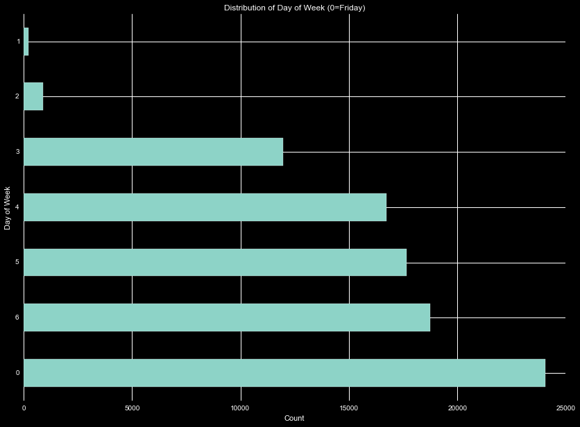
Plotting the date vs logerror by itself showed no long term time variance. However, the date can be converted to a day of the week rather easily. Taking the first date that appears as day 0, and using a modulus operation, we generate a histogram of the count of transactions that occur on a given day. We find that the vast majority of transactions occur on Friday, with almost no transactions on the weekend, and increasing number of transactions leading to Friday. Note the histogram is sorted, so the days of the week are in a semi-chronological order.
Checking the dataset for NaNs and missing data, we see that the variables BuildingClassTypeID, TypeConstructionTypeID, ArchitecturalTypeID, and StoryTypeID contain greater than 99.5% missing values. Considering these are identifications and not amenities, this would leave us with only a few hundred data points to train over. This is not enough for robust classifications, so let's drop the columns.
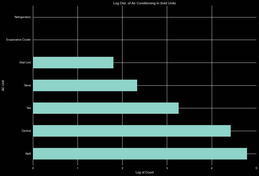
The AC units leaves us room for play. Examining the log of the count of the different AC options, We see there are only one of the purchases with refrigeration and evaporative cooling, and small number listed as wall units or none. We can easily combine the other units into the 'yes' category.
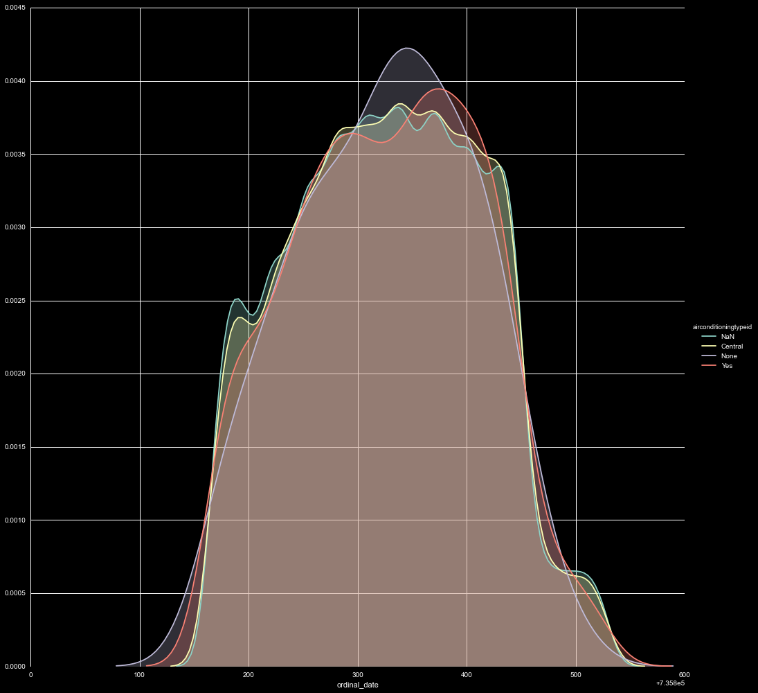
Doing a quick combination of some of the categories, we can look at the kernel of the transaction dates for the different options. It is interesting that the NaNs and 'central air' units show similar peaks and ridges, where the 'yes' and 'none' distributions are more unique. One might expect 'central' and 'yes' to show a similar distribution, and 'none' and NaN categories to overlap more as well. Usually, AC would be advertised as a feature, and in this dataset NaN is commonly used for nothing listed. It is possible these are due to some regional differences. In a hot region it might be important to specify the kind of AC, or list a unit does not have it, where in a cool region it may not be a consideration, and people might not have knowledge of different of AC units. This is absolutely worth following up, and will be continued in further sections.
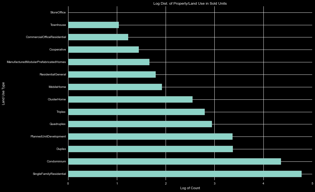
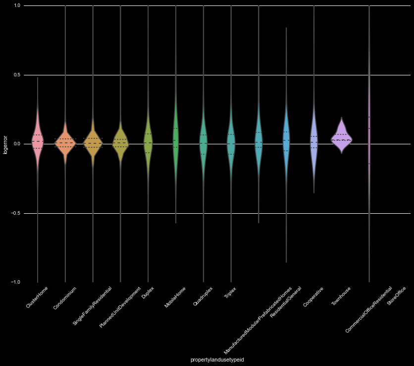
We can next look at the PropertyLandUseTypeID. This has many categories and splits the data set quite a bit between them. While most are residential and may provide easy to combine, there are a few classified as non-residential/offices, and this small number will have to be handled creatively in further analysis.
This is a useful category to compare against the logerror. Generating a violinplot, we see there are some categories with a much higher spread than others-the ones where the number in the sample is small. This can have two possible reasons-the low number in the sample have led to a low significance variation in their distribution, or the low number of these coincides with rarity in their own algorithms, making it difficult to accurately predict the price, and thus the large spread in logerror. We must handle these categories very carfully in our further analysis.
The next variable of interest was HeatingOrSystemTypeID, which is related to the AC unit. The variable distribution was similar as well, with a few odd systems, with 'Yes', 'NaN', and 'Central' as major factors, with a few additional systems in place. There is little difference between their logerror kernels, so we will handle these when we handle the AC units.
Moving onto variables that can be grouped, we start by analyzing pools. The pool data is broken into five variables, three categorical variables: pooltypeid2, pooltypeid7, pooltypeid10, and two continuous variables: poolcnt, and poolsizesum. The three categorical variables have significant overlap, designating pool w/ hottub, pool w/o hottub, and hottub w/o pool. The poolcnt only has two values (NaN and 1), and poolsizesum a total square foot of all pools. Considering the extreme redundancy, we will collapse these into a single categorical variable for if there is a hottub, and the pool square footage. It may be worth including a has pool variable.
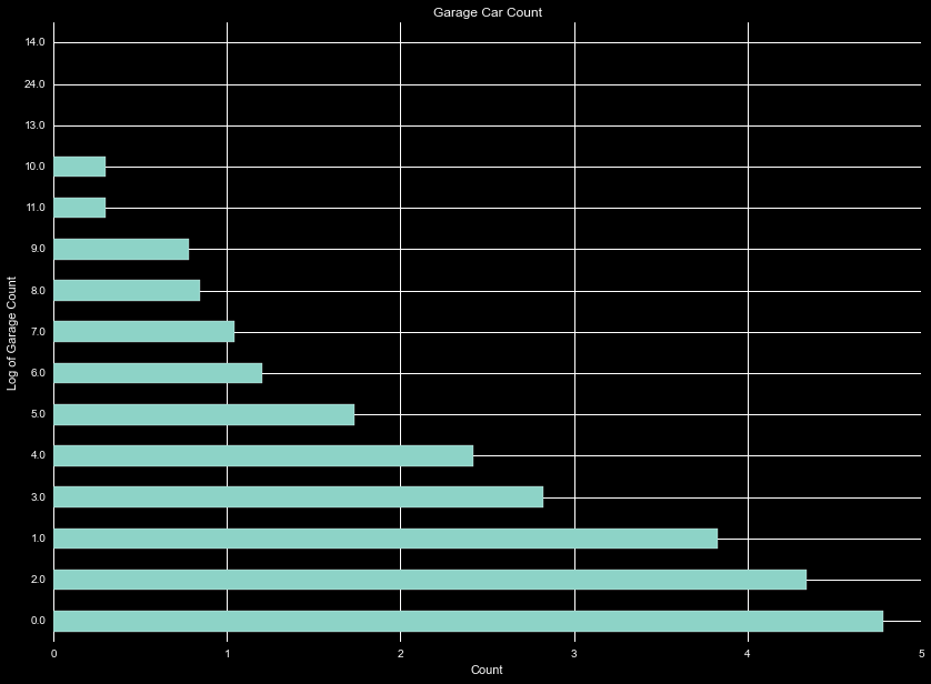
For tracking garages, we see there is a garagecarcount and garagetotalsqft. Needless to say these two show high correlation. Examining the distribution of the log of the count of number of transactions, we see a huge dropoff after about three garages. This may be useful as a categorical variable, or just using the garagesqft variable.
There are several variables tracking bathrooms. Generating a correlation map we see a few trends between them. Namely, two variables are identical, and the fullbathcnt is almost identical to those. Only one variable from this group is needed.

For fireplaces we see more redundant variables. The fireplacecnt contains the number of fireplaces, while the fireplaceflag indicates whether or not there are fireplaces. Drop the flag.
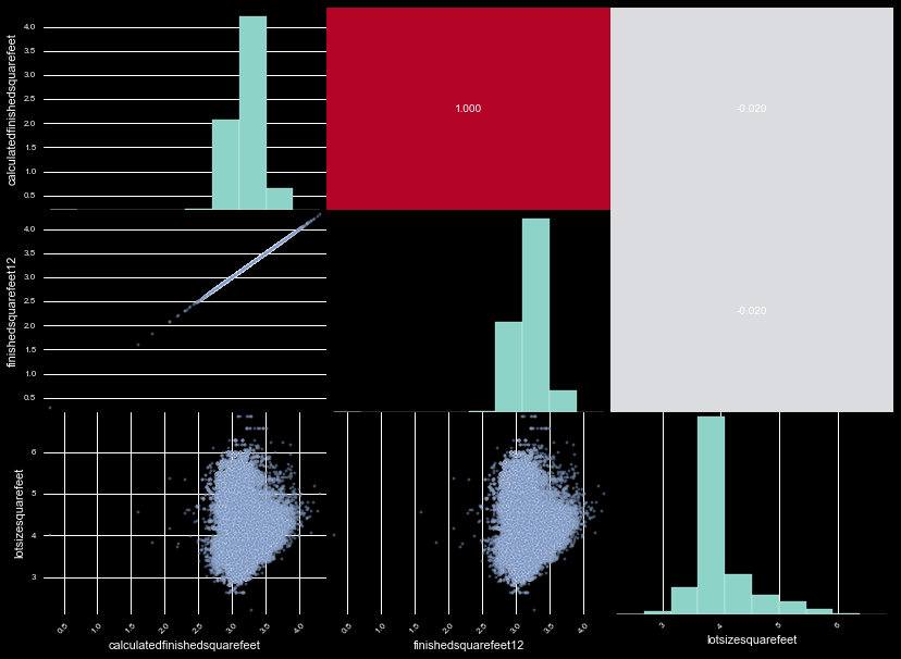
There are roughly 10 variables measuring different square footage, 7 of which contain over 90% NaNs. This makes their usage together very difficult, as we cannot check correlation between the variables. If we use the three with abundant data, we find one variable is a duplicate of the other, and the other completely uncorrelated. This leaves us with two square footage variables independent of eachother, and we don't even have to run PCA analysis.
Looking together at census and assement data, there is a lot to drop. The census track and block variables contain codes used to identify the areas done in the census. There are thousands of these, and there are other, more clear labels in the dataset if we want to use locations. Drop these. Further, these is an assesmentyear variable for the houses, but all are for 2015. Drop.
Next is taxes. There are only about 2000 samples flagged with the taxdelinquencyflag, but that should be enough data to explore. The four tax variables show high correlation, and are perfect for PCA. Logging and rescaling the data, we are able to generate two axes that encompass 96% of the information (85 and 11 percent per axis). This dimensionality reduction will help in future analysis.

Here we are left with a variety of unrelated variables. The propertylandusecodes are
certainly valuable, but there are dozens of codes without explination. While beneficial,
I will not use them further.
The decktypeid has the id number for the style of deck present, but only uses code 66.
This will have to turn into a 1 hot designation.
The numberofstories is mostly 1 or 2, may need to find a good grouping of 3 and 4 together.
Furthermore, this has lots of null values. It may be possible to interpolate values into
the variable.
For regionidcity, regionidzip, regionidneighborhood, we see hundreds of useful codes, all
of thich are difficult to integrate. I will drop them for simplicity.
The buildingqualitytypeid is a scale with high numbers equating low quality, and low numbers
equating high quality. The scale isn't explained and the numbers jump, so we will create
a high, low, medium, and uknown quality classification variable.
Drop the propertyzoningdesc, with thousands of unique codes.
Unitcnt contains the total number of units in a building, can be used to create more categories.
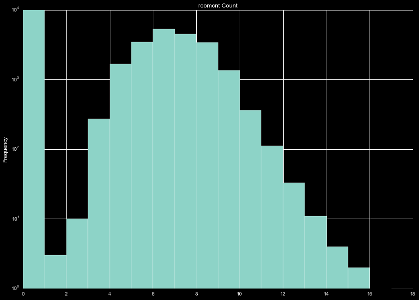
Finally, we can use the roomcnt variable as another continuous variable, and make a flag for
no known rooms (roomcnt=0).
This was designed to be a simple exploratory analysis. Moving forward, I will explore the variables selected in more detail, clean it, and prepare the data for training.