Solar Limb AO
Note: References will be added later, I didn't have them with me at the time I was writing this web page.
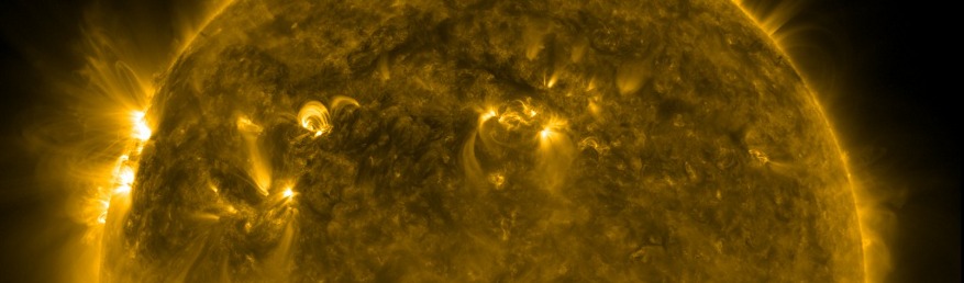
My current research focus is in developing a Solar Limb Adaptive Optics System, under the auspices of Thomas Rimmele, at NSO, in Sunspot, NM.
The challenge with doing adaptive optics on Solar Prominences is that they are comparatively faint. This means that there is very little signal for a Correlating Shack-Hartmann wavefront sensor. Our first attempt at measuring wavefront involves using very large subapertures, thus dividing the main telescope beam into relatively few parts. This allows for more light throughput per subaperture, at the cost of detail in wavefront reconstruction.
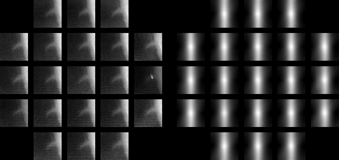
Here's what some of the data look like:
On the left are images of each subaperture, arranged with respect to each area of the telescope aperture that they represent. On the right, are the cross correlation plots taking one of the subapertures in the first frame as a reference. One can see how atmospheric turbulence causes the images to move relative to each other. The brightest points in the right-hand images show the absolute position of the image in each subaperture, relative to the afore mentioned reference. Note: the animations below contain only the first 15, out of 100 frames, in this particular set of data.
Once the position of each subaperture, for each frame, is measured, the relative positions can be used to reconstruct the wavefront of the light that enters the telescope. A perfect wavefront would be completely flat. (And we would observe no motions of subapertures.) An aberrated (distorted) wavefront will appear to have peaks and valleys. In the image below, one can see the reconstructed wavefronts, corresponding to the image motion shown in the above animation. Black corresponds to valleys, which are approximately 5 wavelengths of 550nm light lower than average (green). Red corresponds to peaks, 5 wavelengths higher than average.
At this point, it is necessary to explain how the wavefront is actually measured. The wavefront can be stated in terms of a linear combination (IE, addition of each item, times a unique constant, a coefficient.) of Zernike Polynomials. These polynomials describe various optical aberrations. The above animation was constructed from the Zernike Polynomials, times their unique coefficients, which were measured from the image positions, measured earlier. So what, you say, am I measuring anything real, or is this all spurious noise? It turns out that there is a model for atmospheric turbulence, called the Kolmogorov model. Following this model, it is possible to determine how much the coefficients of each Zernike Polynomial should change, for a given degree of atmospheric turbulence. (their variance) It is then possible to compare the measured variance of each coefficient, with their expected variance, in order to see if I am measuring anything real.
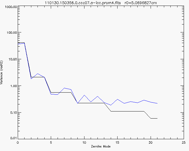
One can see, then that my data behave close to the way they should, up until we hit mode #13, after which, things go to pot. One should note that the value r0, mentioned in the plot above is called the Fried Parameter. It states the size of a telescope aperture, over which the wavefront is distorted by only 1 radian (that is, one wavelength of light, at 550nm, divided by 2 times Pi). r0 is found from fitting the data, blue, to the expected line. Note that r0 is the only free parameter in this fit and it only moves the black line vertically, relative to the blue one. If the measured wavefronts were spurious, no value of r0 would make the date fit the expected line. The above data are some of the best that I have measured so far. Here is an example of very poor data:
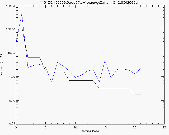
As you can see, the data do not fit the graph well at all. Below is a single frame, which will aid me in explaining why. Notice how the right hand images are vertical lines, that is because, this image is mostly the bright edge of the sun and it is easy for the computer to determine position left to right, but very difficult for it to see up and down. This is because that little Prominence has very low contrast, relative to the rest of the image. Also, the Solar Limb spans the whole image, from top to bottom compounding the difficult in measuring shifts in the vertical direction.
This shows one of the difficulties with Solar Limb AO, it works best with very high contrast, highly detailed Prominences. In the future, we plan to test a technique called Phase Diversity, which will aid in getting high contrast images, and thus, good wavefront measurements.