A common, or base 10, logarithm is the exponent e to which you raise the number 10 in order to match a certain value (x). We raise 10 to the third power in order to make it equal to 1,000, so the logarithm of 1,000 (or 10) is 3; we raise ten to the second power to match 100, so the logarithm of 100 (10) is 2; and we raise ten to the first power to match itself, so the logarithm of 10 (10) is 1.

This pattern continues as we raise ten to the power of –1 to match 0.1 (10), and we raise ten to the power of –2 to match 0.01 (10). Can you think of an exponent e to which you can raise ten which will equal a negative number (some e for which 10^e = x when x < 0)? We can't either, which is why we can only take logarithms for positive numbers (x values greater than zero). When e itself is positive, x is greater than 1, and when e is negative, x lies between 0 and 1.

When we plot data, we can chose to use linear or logarithmic axes. A linear plot has linear axes, where as you shift across the plot by set amounts you keep adding the same amount. A logarithmic plot has logarithmic axes, so as you shift position by set amounts you keep multiplying by the same factor. Linear axes are useful when your data are all grouped together with roughly equal spacing, while logarithmic axes allow you to compare data points drawn from a wide range simultaneously (on a single plot).

Example
Let's look at an example of a linear plot and a logarithmic plot of the same relationship. In this case, size is a function of age, and older structures are larger. If we know a structure's age, we should be able to read off its predicted size from our plots. As we shall see, a logarithmic plot can be easier to read than a linear one in some cases. A set of points have been added spanning the entire range in age; note how the points are spaced out on the logarithmic plot but bunch up on top of each other at one end of the linear plot.

Linear Plot of Size versus Age

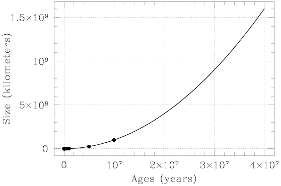This figure contains a linear plot showing a relationship between age, in years, and size, in kilometers. As we move along the horizontal axis from labeled point to labeled point, we add 10 million years with each step (moving from 10 to 2 × 10, and then to 3 × 10, and so on). The total range in age is 40 million years. It is easy to determine the size values from the vertical axis for ages greater than ten million years, but more difficult to determine behavior for smaller ages. Note that the tick marks between each labeled point along the axes are equally spaced. Between 10 and 2 × 10, the 4 equally spaced marks take on values of 1.2 × 10, 1.4 × 10, 1.6 × 10, and 1.8 × 10, as we keep adding on another 2 million years.

Logarithmic Plot of Size versus Age

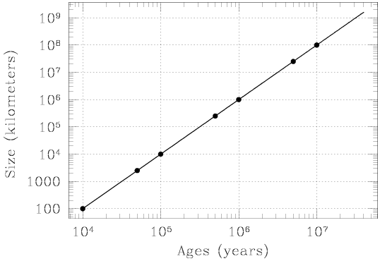This figure contains a logarithmic plot showing a relationship between age, in years, and size, in kilometers. The relationship between age and size is the same as for the linear plot. As we move along the horizontal axis, we multiply the age by a factor of ten with each step (now moving from 10 to 10 to 10, and so on). The total range in age is still 40 million years, but an equal amount of space along the horizontal axis is devoted to the interval between one million and ten million years and that between 100,000 and one million years, and between 10,000 and 100,000 years. This makes it easy to to read off size values for both large and small ages. The 8 tick marks between each set of labeled points correspond to multiplying by factors of 2, 3, 4, 5, 6, 7, 8, and 9. Between 10 and 10, they take on values of 2 × 10, 3 × 10, 4 × 10, and so on up to 9 × 10. Note that the distance between 10 and 2 × 10 is equal to the distance between 2 × 10 and 4 × 10, because in each case we multiplied by a factor of two.

If we placed a ruler on top of the linear plot, and kept moving a set distance along the horizontal axis, we would keep adding the same amount. In contrast, if we then placed it on top of the logarithmic plot and kept moving a set distance, we would keep multiplying by the same amount.

Try to determine the size of an object which is one million (10) or 100,000 (10) years old, first on the linear plot and then on the logarithmic plot. Though both plots show the same relationship over the same range, it is remarkable how much easier it is to determine the size values from the logarithmic plot!

Here is a short video about logarithms for further review.