The scientific method plays a significant role in conducting experiments, along with good experimental technique and basic statistics. Laboratory experiments will help you to better understand how scientists test their hypotheses. Here are a few reminders concerning some of the basic statistics used in laboratory experiments.

Histograms and normal distributions (μ and σ)
We often measure a certain quantity for a subsample of objects, and apply the results of our investigations to a larger population. We might weigh the contents of 30 randomly chosen cans of soup in order to estimate the average weight of a bowl of soup, or measure the luminosity of 30 stars with the same surface temperature as that of the Sun in order to estimate the average luminosity of G-type stars.

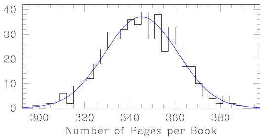
When we have built up a large number of repeated measurements of the same quantity, we can bin the data (counting up how many measurements fall within each bin width), and plot the results in a histogram. Here is a histogram showing the distribution of book lengths for 500 novels.

The average value, or the sum of the measurements divided by the number of measurements, is called the mean value (μ). Note how the number of books per bin rises from both sides as we approach the mean value (345 pages). The smooth blue curve is called a normal curve, or bell curve, and shows what the distribution would tend to look like if we had a large number of measurements made to very high accuracy.

Once we have defined the mean value of our measured quantity, the next logical question is how scattered our measurements are around the mean. Do they cluster closely, or do we find a large variation in book lengths? Sigma (σ) is a measure of how much the individual measurements differ from the mean value, on average. The larger the σ value, the more widely distributed the measurements will be.

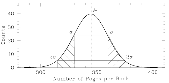Two-thirds of the measurements should lie within 1σ of the mean, in the inner white region between the x-values of μ–σ and μ+σ in the plot shown above. A deviation of 1σ is quite typical. As we move further away from the central value, we observe that 95% of all measurements should lie within ±2σ of the mean (within the inner white region and the two hatched side regions). A mere 5% of all measurements will lie more than 2σ above or below the mean value. If you compare two sets of measurements of a given quantity and find that the difference between their mean values is more than 3σ, you should investigate whether there may be differences in the experimental technique (or in the definition of the measured quantity).

Errors
Consider three types of errors.

1. Measurement error is defined by the precision of our equipment. If we used a stopwatch which only shows seconds, then time interval measurements might be recorded to the nearest second. Each value could be 0.5 seconds lower, or 0.5 seconds higher, than the recorded value.

2. Systematic errors are errors in experimental design which act to bias all measurements in the same way. If we measured how well people could see but forgot to ask them to take off their glasses and contact lenses first, then we would think that the human eye worked better than it does.

3. Natural variation refers to the innate width of the distribution of a measured quantity. Even with perfect measuring tools, we would not measure the exact same value for every object within a sample for a given quantity. (For example, people have feet of different lengths, and galaxy disks have different sizes.)