Defining a Straight Line

Good science depends critically upon solid data analysis. Let's look at an example of this, by considering functions that can be fit with a straight line. If we know the relationship between two variables x and y, then if we know x we can predict the value of y. (The values for y and x could be anything – peak temperature versus day of the year, lunar phase versus day of the lunar month, height versus age, ...).

If you know the position of two points in space, there is one and only one line which will pass through them both. (Test this idea for yourself, by marking two points on a piece of paper and trying to draw two different straight lines through them.) We can say that these two points are defined by their x and y coordinates (x,y), their location to the left or right (x) and upwards or downwards (y) of a starting point, or origin.

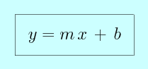
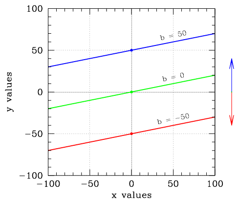
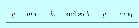
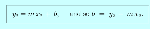
We often define a line in terms of two variables. The first is its slope, the amount by which its position increases in y as we increase x, often called m. The second is its y-intercept, the y coordinate along the line for which x is equal to zero, called b.

Equation for a line: y is equal to m times x plus b.

In the equation shown above, what value does y have if x is set equal to zero?

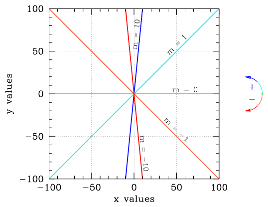
The slope of a line tells you how tilted it is. The larger its slope, the more a line tends toward a pure vertical, while a line with a slope of zero is a horizontal line. A line with a large, negative slope also tends toward a vertical, but descends rather than ascending. This figure shows five different lines (each one drawn in a different color). The bluer the line, the higher the slope, and as the lines shift toward redder colors, the slopes shift down toward negative infinity.
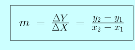
Scatter plot showing the region where x (on the horizontal axis) varies from -100 to 100 and y (on the vertical axis) varies from -100 to 100. A horizontal green line is labeled m (the change in y divided by the change in x) is equal to zero; a light blue line at a 45 degree angle running up from (-100,-100) to (100,100) is labeled m is equal to 1; an ascending almost vertical dark blue line is labeled m is equal to 10; a descending almost vertical dark red line is labeled m is equal to -10; a light red/orange line at a 45 degree angle running down from (-100,100) to (100,-100) is labeled m is equal to -1.

The following figure shows three more lines, with the same slope but different y-intercept points. As the y-intercept shifts upward from zero (the green line), the entire line shift along with it (blue line). If instead the y-intercept shifts downward from zero, the entire line drops down with it (red line). You can read the y-intercept values right off of the plot, by finding the y-value for each line at the point at which x is equal to zero. (These three points are drawn as dots on the plot.)

Scatter plot showing the region where x (on the horizontal axis) varies from -100 to 100 and y (on the vertical axis) varies from -100 to 100. A slightly tilted green line running through the point (0,0) is labeled b (the y-intercept) is equal to zero; a similarly tilted blue line above running through the point (0,50) is labeled b is equal to 50; a similarly tilted red line below running through the point (0,-50) is labeled b is equal to -50.

If we know the coordinates of two points – (x1, y1) and (x2, y2) – along a line, we can calculate its slope and its y-intercept from them. The slope, m, is the change in y (The Greek letter Delta.y, or y2 - y1), divided by the change in x (The Greek letter Delta.x, or x2 - x1).

Equation for the slope of a line: m is equal to Delta-Y divided by Delta-X, which is equal to the quantity ( y2 minus y1 ) divided by the quantity ( x2 minus x1 )..

The y-intercept can be found by combining x1, y1, and m, or by using x2, y2, and m. We know that

Equation for the y-intercept of a line: y1 is equal to m times x1 plus b, and so b is equal to y1 minus m times x1.

and so it is also true that

Equation for the y-intercept of a line: y2 is equal to m times x2 plus b, and so b is equal to y2 minus m times x2.

When we fit a line to a set of data points, we define the root mean square (rms) deviation of the line as a quantity built by combining the deviation (the offsets) of each of the points from the line. The higher the rms value for a fit, the more poorly the line fits the data (and the more the points lie off of the line).