|
Slides for NGC 891 and NGC 4631 - 21 July 2014
NGC 4565
| |
 |
|
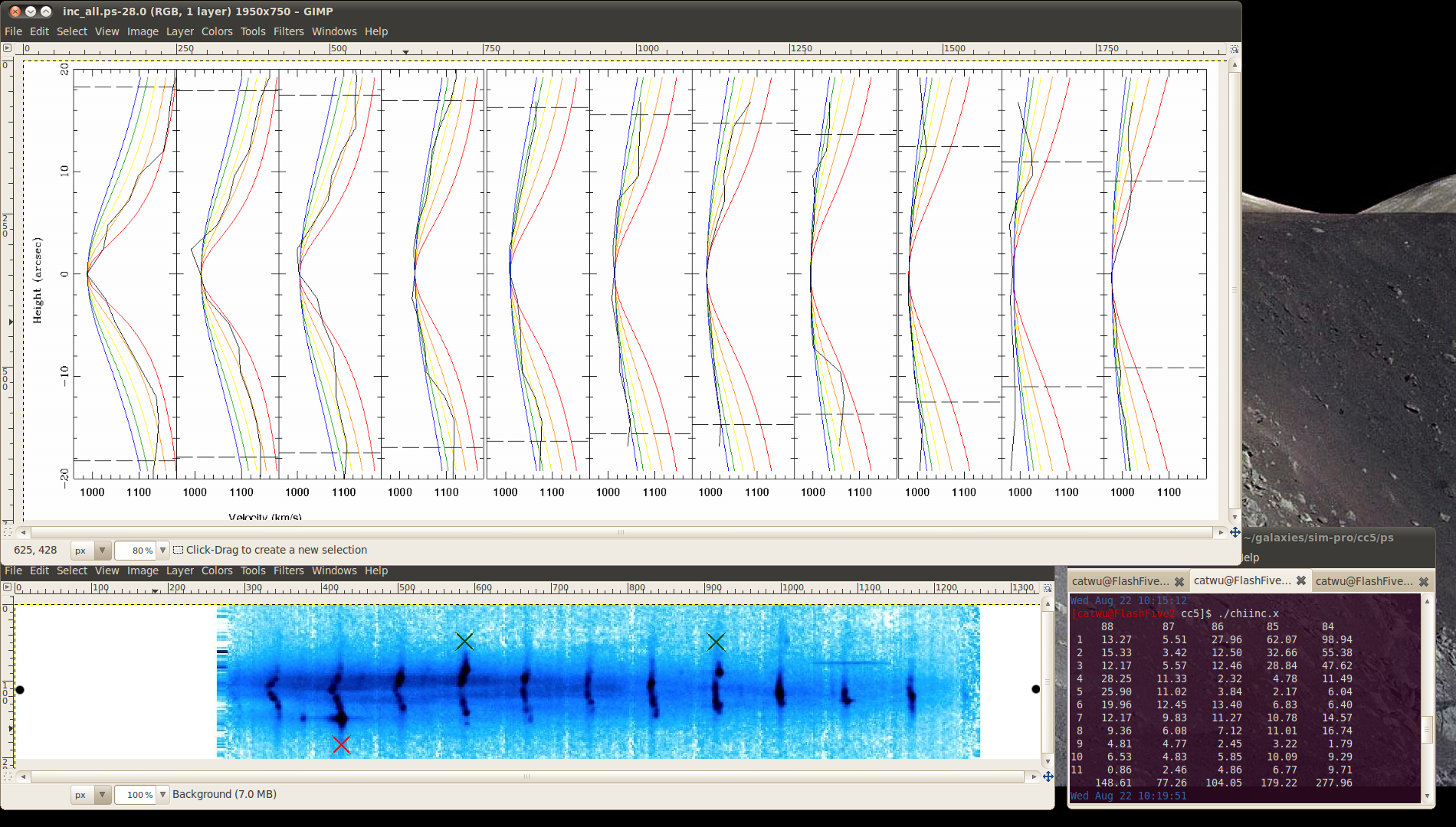
Simulating the observed emission profile as seen through an edge-on disk... The code is set up so the user can specify the vertical rotational velocity gradient, height range above the disk, density profile of the gas (constant or 1/e-r) in radial- and z-directions, systemic velocity of the galaxy, and rotation curve (in the form of an equation or text file). | |||||||||
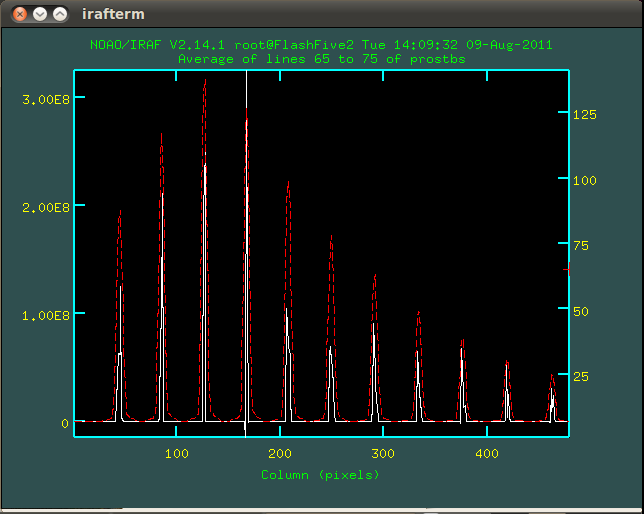
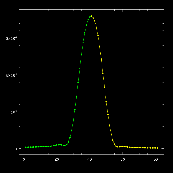
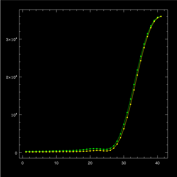
| The red line in the top plot is a cut across the simulated spectrum after convolving each slit with the same kernel, then wavelength-calibrating and reducing the dispersion to 0.57A/pix. The white line is the same cut on the non-convolved spectrum (after wavelength-calibrating and reducing the dispersion). The kernel was generated by taking the average of the middle 5 lines of the observed arc frame, splitting it into 11 separate profiles, shifting the 11 profiles so their peaks match, and then taking the average of the 11 profiles. The peak of the kernel is in the center of the kernel. The profiles of the convolved spectrum match up with those of the non-convolved spectrum, so convolving with this kernel does not appear to introduce a shift in the spectrum. However, while the kernel has its peak in the center, the profile is not symmetric. The lower left plot shows the average kernel taken from all 11 profiles. The lower right plot shows this kernel folded in half.
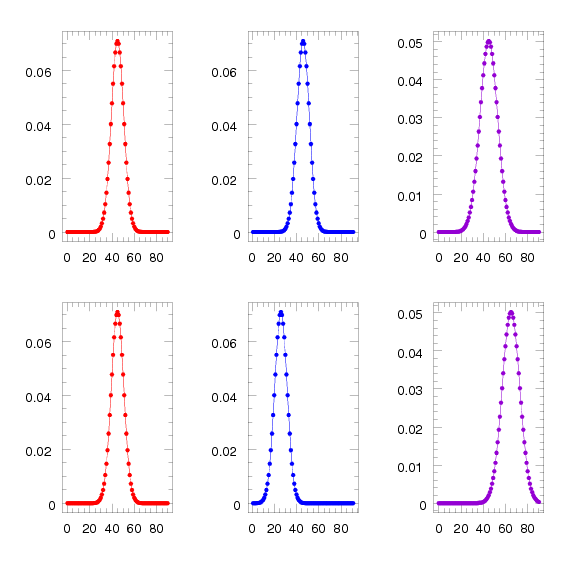
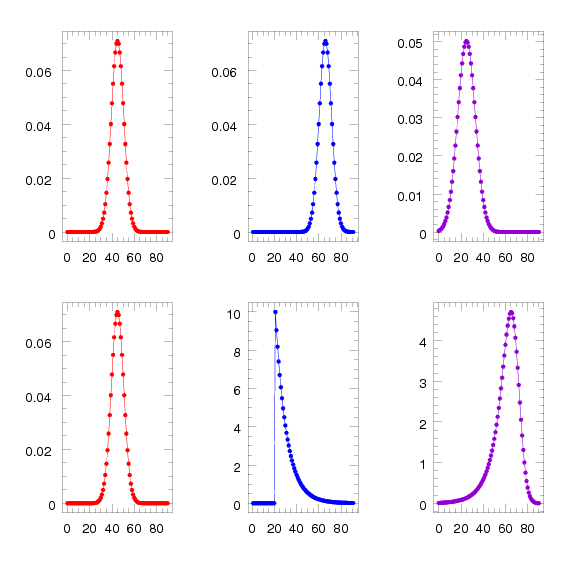
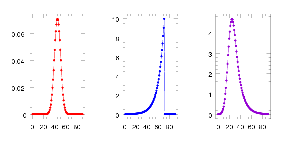
| IRAF's CONVOLVE task takes a fits file and convolves it with a kernel in the x-direction specified by a text file. In general, the kernel needs to be flipped about the y-axis before convolving it with the fits file. The CONVOLVE task does not flip the kernel, so the specified text file must contain the reverse of the desired kernel. The plots below show the result (purple) of a gaussian (red) convolved with different kernels (blue). The kernels are a centered gaussian, a gaussian offset to the left, a gaussian offset to the right, a non-symmetric function offset to the left, and a non-symmetric function offset to the right.
| HI pv diagram from Rand, 1994. Systemic velocity for NGC 4631 is 606-610 km/s. From Rand's plot, I assumed that the maximum rotational velocity on both the east and west sides of the galaxy is systemic +/- 150 km/s and that the rotation curve flattens at that velocity at +/- 1 arcmin from the galaxy's center. I also assumed that between -1 and +1 arcmin, velocity as a function of radius is a linear relation. Any velocities between -1 and +1 arcmin fall along the line connecting the points (-1 arcmin, 760 km/s) and (+1 arcmin, 460 km/s), and the velocity for radii outside that range is 460 or 760 km/s. My simulated galaxy disk for 4631 cuts off at +/- 9 arcmin.

Observed LOS velocities. The at_r values listed in the upper right corner are the LOS radii in arcmin. The values (in arcmin) are 0.0, 0.2, 0.4, 0.6, 0.8, 1.0, 3.0, 5.0, 7.0, and 9.0. At LOS radius of 0, measured velocity will be systemic velocity (the plot says 0 km/s because this was run with v_systemic = 0 km/s to check that it was the same as running for v_systemic = 610 k/ms) since rotational velocity is all perpendicular to the observer's LOS. Looking at LOS radii farther and farther from the center (red - orange - yellow - green - blue), the observed velocity increases as long as LOS radius is less than the radius at which the rotation curve flattens (solid body rotation regine). At LOS radii where the rotation curve is flat, the observed velocity is always 150 km/s (v_flat in this case) at the tangential point (midplane).
| For a given LOS radius, observed velocity is flat in the inner part of the disk because as y (pathlength, which affects distance from center) increases, rotational velocity increases (due to solid body rotation), but the velocity component along your LOS decreases, and the two cancel out. The observed velocity is flat until radius equals 1 arcmin, which is radius at which vel curve flattens for 4631. As LOS radius increases, the y-value (pathlength from midplane) at which radius equals 1 arcmin decreases. Because this is plotted as a function of y (and not radius), the drop-off point is lower and lower and LOS radius inreases. The value on the x-axis is how far you're looking through the galaxy - at the galaxy center, you're looking through the entirety of the galaxy (0 to 9 arcmin in this case), but farther out, your LOS intersects a smaller section (pathlength) of the galaxy. 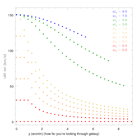
Observed LOS Velocities with a lagging halo Similar to the plot above, except the x-axis is radius from the center of the galaxy instead of y (pathlength through the disk). Each color corresponds to a different height above the disk (with green being the midplane) for a lag of 20 km/s/kpc. For LOS radii interior to radius = 1 arcmin (where velocity flattens), the green line shows constant observed velocity because of solid body rotation (explained for the plot above). The other heights show an increase in observed velocity in the solid-body rotation part of the disk. This is because applying a lag (subtracting a constant from the velocity at each radius) to the velocities means you no longer have solid body rotation. For 4631's rotation curve and a lag of 20 km/s/kpc, the rotational velocity increases more than the velocity component along your LOS decreases, so the result is the inreasing LOS velocity from r = 0 arcmin to r = 1 arcmin. After r = 1 arcmin, the observed velocity drops off. |
The bottom right plot (LOS radius = 3 arcmin) has steeper velocity dropoff than the bottom middle plot (LOS radius = 6 arcmin) because at smaller LOS radii, as you look through the pathlength along your LOS, the observed velocity goes from tangential (at the midplane) to almost systemic (most of rotational velocity is perpendicular to your LOS). At larger LOS radii, observed velocity alaso starts at tangential (at the midplane). But at the edge of the disk, most of the rotational velocity is still along your LOS (or, less of it is perpendicular compared to LOS radii closer to the center). So the decrease in observed velocity is less at larger LOS radii. 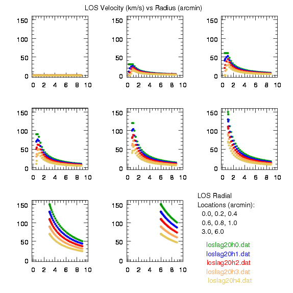 | |||||
|
| ||
 | ||
|
| ||
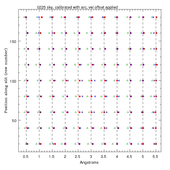 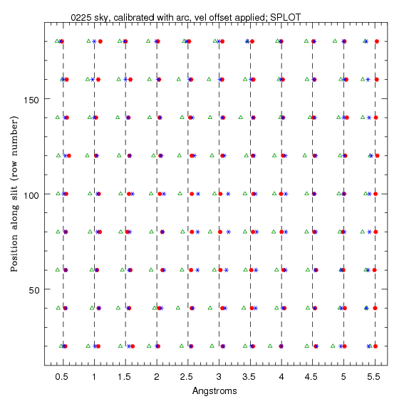 | ||
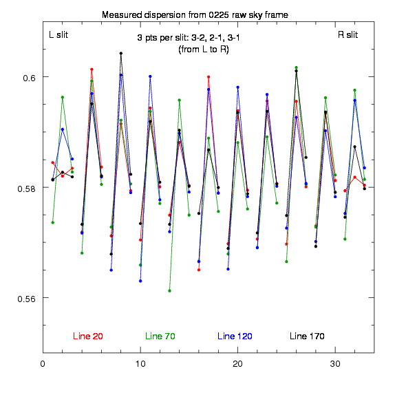 0225: disp3-1 = 0.5802 disp3-2 = 0.5712 disp2-1 = 0.5938 |
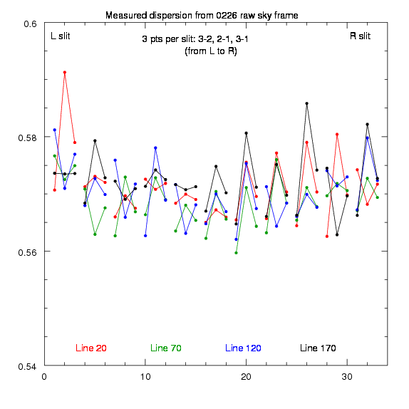 0226: disp3-1 = 0.5701 disp3-2 = 0.5682 disp2-1 = 0.5730 |
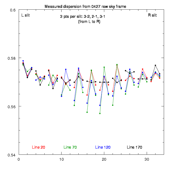 0427: disp3-1 = 0.5705 disp3-2 = 0.5690 disp2-1 = 0.5726 |
|
| ||
|
IRAF 'implot' task... linear background, the peak position and distance from the background and the widths at half the peak value are overplotted on the data. In addition to the profile quantities the moments of the background subtracted data are measured. The moments computed are the centroid, the integral (or flux), the width, and the normalized asymmetry. The width reported is the square root of the second central moment multiplied by 2.35482. For a gaussian profile this corresponds to the full width at half maximum which can be compared with the direct measure of the profile width. The normalized asymmetry is the third central moment divided by the 3/2 power of the second central moment. The various measurements are printed on the status line. There are multiple lines of results which are scrolled using the '/' key. |
|
Mysteries of (An)amorphic (De)Magnification...
Schweizer, Francois: Anamorphic Magnification of Grating Spectrographs - A Reminder
Christlein, D. and Zaritsky, D. The Kinematic Properties of the Extended Disks of Spiral Galaxies: A Sample of Edge-on Galaxies
Slit Width Selection (from NOAO)
Here w is the projected slit width, W the actual (physical) slit width, and r is the "grating anamorphic magnification". The factor r is a function of the grating tilt and collimator-camera angle, i.e. where phi is the collimator-camera angle (46 degrees) and t is the grating tilt. For the UV Fast Camera, the camera-to-collimator focal ratio is ~0.23 . At large grating inclinations the anamorphic demagnification factor becomes significant. In these cases the slit can be opened slightly wider without degrading the resolution. See F. Schweizer's article PASP 91, No. 539, 149, 1979 for more information.
|
|
IRAF Lingo...
combine = "average" (average|median|sum)
reject = "none" (none|minmax|ccdclip|crreject|sigclip|avsigclip|pclip)
scale = "none" (none|mode|median|mean|exposure|@
zero = "none" (none|mode|median|mean|@
weight = "none" (none|mode|median|mean|exposure|@
statsec = ""
SCALES AND WEIGHTS
Examples of the possible parameter values are shown below where
"myval" is the name of an image header keyword and "scales.dat" is
a text file containing a list of scale factors.
The image statistics are computed by sampling a uniform grid of
points with the smallest grid step that yields less than 100000
pixels; sampling is used to reduce the time needed to compute the
statistics. If one wants to restrict the sampling to a region of
the image the statsec parameter is used. This parameter has the
following syntax:
The statistics are as indicated by their names. In particular, the
mode is a true mode using a bin size which is a fraction of the
range of the pixels and is not based on a relationship between the
mode, median, and mean. Also masked pixels are excluded from the
computations as well as during the rejection and combining
operations.
The "exposure" option in the intensity scaling uses the value of the
image header keyword specified by the expname keyword. As implied
by the parameter name, this is typically the image exposure time
since intensity levels are linear with the exposure time in CCD
detectors. Note that the exposure keyword is also updated in the
final image as the weighted average of the input values. Thus, if
one wants to use a nonexposure time keyword and keep the exposure
time updating feature the image header keyword syntax is available;
i.e. !
Scaling values may be defined as a list of values in a text file.
The file name is specified by the standard @file syntax. The list
consists of one value per line. The order of the list is assumed
to be the same as the order of the input images. It is a fatal
error if the list is incomplete and a warning if the list appears
longer than the number of input images. Because the scale and zero
levels are adjusted only the relative values are important.
If both an intensity scaling and zero point shift are selected the
zero point is added first and the the scaling is done. This is
important if the scale and offset values are specified by header
keywords or from a file of values. However, in the log output the
zero values are given as the scale times the offset hence those
numbers would be interpreted as scaling first and zero offset
second.
The image statistics and scale factors are recorded in the log file
unless they are all equal, which is equivalent to no scaling. The
scale factors are normalized so that the first input image has no
scaling. This is done because the header of the first input image
is used as the template header for the combined output image. By
scaling to this first image this means that flux related keywords,
such as exposure time and airmass, are representative of the output
(except when the "sum" option is used).
Scaling affects not only the mean values between images but also the
relative pixel uncertainties. For example scaling an image by a
factor of 0.5 will reduce the effective noise sigma of the image at
each pixel by the square root of 0.5. Changes in the zero point
also changes the noise sigma if the image noise characteristics are
Poissonian. In the various rejection algorithms based on
identifying a noise sigma and clipping large deviations relative to
the scaled median or mean, one may need to account for the scaling
induced changes in the image noise characteristics.
In those algorithms it is possible to eliminate the "sigma
correction" while still using scaling. The reasons this might be
desirable are 1) if the scalings are similar the corrections in
computing the mean or median are important but the sigma
corrections may not be important and 2) the image statistics may
not be Poissonian, either inherently or because the images have
been processed in some way that changes the statistics. In the
first case because computing square roots and making corrections to
every pixel during the iterative rejection operation may be a
significant computational speed limit the parameter sigscale
selects how dissimilar the scalings must be to require the sigma
corrections. This parameter is a fractional deviation which, since
the scale factors are normalized to unity, is the actual minimum
deviation in the scale factors. For the zero point shifts the
shifts are normalized by the mean shift before adjusting the shifts
to a zero mean. To always use sigma scaling corrections the
parameter is set to zero and to eliminate the correction in all
cases it is set to a very large number.
If the final combining operation is "average" then the images may be
weighted during the averaging. The weights are specified in the
same way as the scale factors. In addition the NCOMBINE keyword,
if present, will be used in the weights. The weights, scaled to a
unit sum, are printed in the log output.
The weights are used for the final weighted average, sigma image,
and exposure mask output. They are not used to form averages in
the various rejection algorithms. For weights in the case of no
scaling or only multiplicative scaling the weights are used as
given or determined so that images with lower signal levels will
have lower weights. However, for cases in which zero level scaling
is used and the zero levels are determined from image statistics
(not from an input file or keyword) the weights are computed from
the initial weights (the exposure time, image statistics, or input
values) using the formula:
The weights are not adjusted when the zero offsets are input from a
file or keyword since these values do not imply the actual image
sky value. In this case if one wants to account for different sky
statistics in the weights the user must specify the weights in a
file taking explicit account of changes in the weights due to
different sky statistics.
When forming the final weighted averages if the sum of the weights
of the non-rejected or excluded pixels is zero then instead of
producing a zero average the unweighted average of the pixels is
produced. Similarly, in the sigma calculation when the weights of
the pixels are all zero then the sigma is computed as if all pixels
have unit weights.
When there are zero weights only the pixels with non-zero weights
are used in computing the output exposure time mask. Note that the
actual weight values are not used but simply the sum of all
exposure times of pixels from images with non-zero weights is
produced.
The purpose of using zero weights is to identify images that are of
poor quality (such as non-photometric or bad seeing) which are then
excluded in the final weighted average or exposure time. However,
they contribute to the final image when there is no good quality
data but with an output exposure time of zero.
|
| NMSU Astronomy | Fall 2014 | Cat Wu |