Nbody

Simulations with direct summation codes

This is an example of top-hat collapse. Initial sphere has homogeneous distribution (top left plot). Initial random velocities are very small: kinetic energy is 1 percent of the total energy. The system starts collapsing. After a short and very violent crossing (the second and third rows of plots) the system relaxes and develops quasi-equilibrium distribution (bottom row). The equilibrium region grows very fast in radius just after the crossing. Then its growth slows down as the equilibrium radius reaches peripheral region, where the time-scale of evolution is getting longer and longer.

The period of crossing is very important and consists of two stages: before and after the moment of maximum contraction. During the infall stage the system is unstable on all scales. Different non-spherically symmetric perturbations develop before the crossing. The right plot in the second row from the top shows very strong perturbations inside the collapsing region. The situation drastically changes after the crossing. There is a very strong exchange of energies between particles and perturbations, which results in some particles losing the energy (those, which came before the crossing) and some getting the energy. The large-scale animation gives an impression of an explosion: some fraction of particles get very large velocity and quickly leave the central region.

Diameter = 4 initial radii	Diameter = 1 initial radius

The simulation has 50,000 equal-mass particles. The force softening is 0.001 in units of the initial radius of the sphere. The code uses variable-step drift-kick-drift numerical scheme. The energy is preserved with 1e-5 accuracy during the whole evolution

Particles are split into groups based on their velocities: displacements of particles per each time step deviate less than a factor of two. All particles in a group move with the same time-step. After all particles finish the largest (zero-level) step, assignment of particles to groups may change. During the assignment a particle may change its time-step only by factor two. The code is parallelized using OpenMP directives. The scaling was nearly perfect for 30 processors.

LowResMovie: diameter of the image is 4 initial radii. High-res movie

HighResMovie Movie with zoom into the central region: diameter is 1 Initial radius. Note that fluctuations and deviations from spherical symmetry grow dramatically during the initial infall stage. The fluctuations are quickly disappearing immediately after the first crossing.

Images: ViewHighRes HighResZoom

		Tests of integration of trajectories. System has two equal mass particles moving on a perfect highly elliptical orbit. Orbit eccentricity is e=0.9, which gives the apocenter/pericenter = 11. It is a difficult test for time-stepping schemes. The acceleration changes more than 100 times. Most of the change happens during a short period of time when the particles are close to pericenter. Slight asymmetries in integration may result in a large change of total energy. Time-symmetric leapfrog scheme preserves the energy, but it gives significant drift in the orientation of the orbit. Another issue is accuracy of integration over a very long period of time. Code must provide accurate solution for many thousands of orbits.
		Mass of each particle is 1. Particles start at apocenter, which is set to 1. Period of the orbit is 4.8. Force softening=0

Energy conservation (top panel) and drift of orbit orientation (bottom panel). Initial orbit is shown with the full curve.
The dotted curve shows the trajectory after 1000 periods.

Variable step with 1500 accelerations/period.

Simulations with variable time-step. Parameters: dt=5.e-3, 1500 estimates of acceleration per orbit. Max number of refinement levels =4, displacement per step 1.e-2, relative change of velocity per step=1.e-2

		The same test, but on much longer time-scale: 100,000 orbits. Number of force estimates per orbit is 3000. The bottom panel shows every 10000 orbit. There is significant drift in the orientation of the orbit, but not systematic change in the energy.
		Simulations with variable time-step. dt =2.5e-3,relative change in velocity per time-step is 5e-3, change of coordinates per time-step is 5e-3

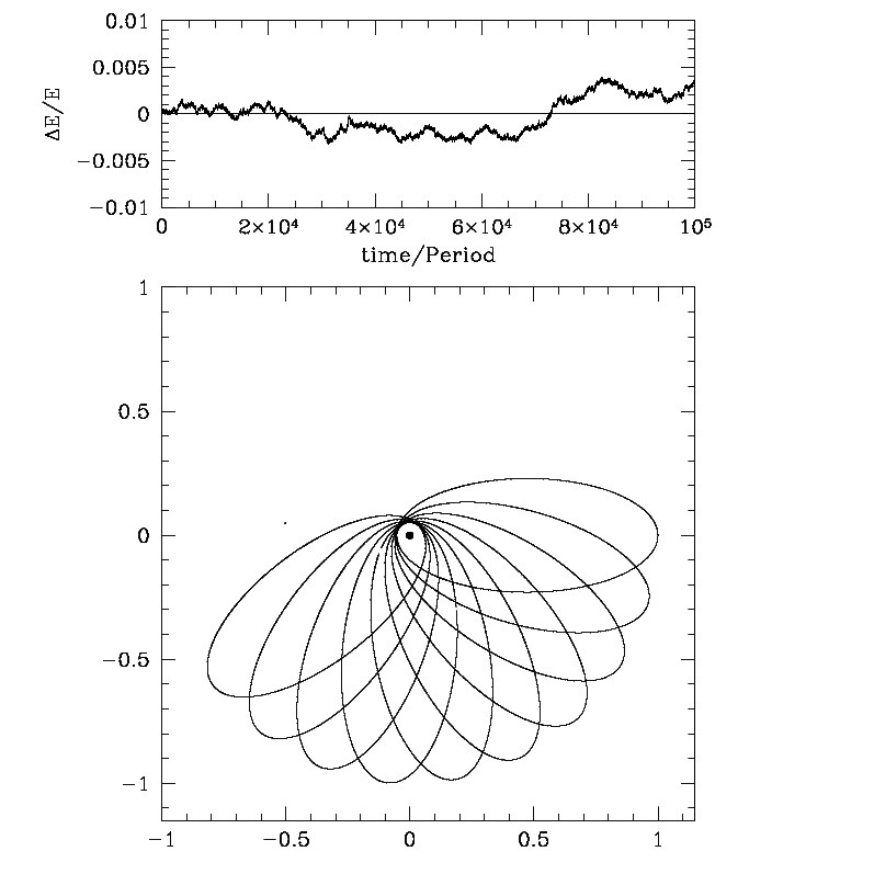
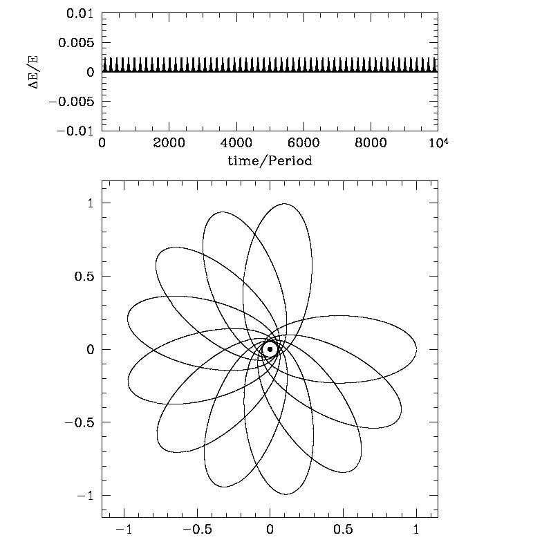
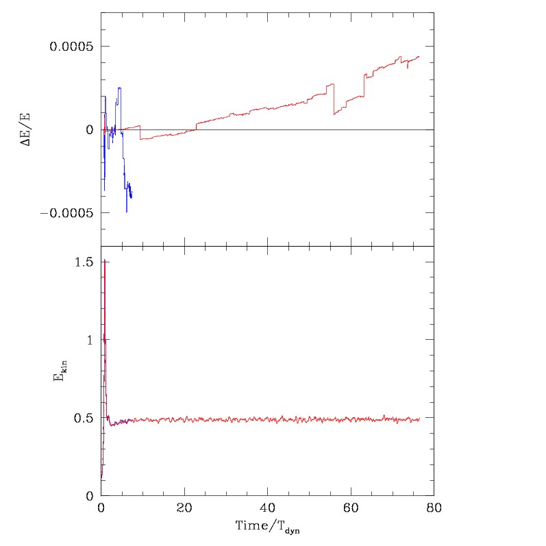
The same as the first plot, but done with constant time-step. Thus, this is pure leapfrog integration with the same force estimates per orbit: 1500. The energy conservation is better for variable time step for the first 5000 orbits. After that it gets to the same level as leapfrog. If the same test runs for 50,000 orbits, than energy gets worse for variable time-step - about dE/E=0.01. Increasing the accuracy by factor two (as in the plot above) gives accurate solution for at least 100,000 orbits.

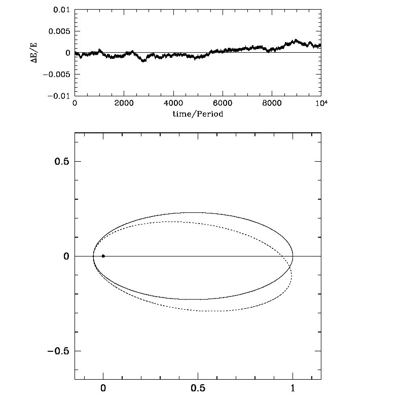
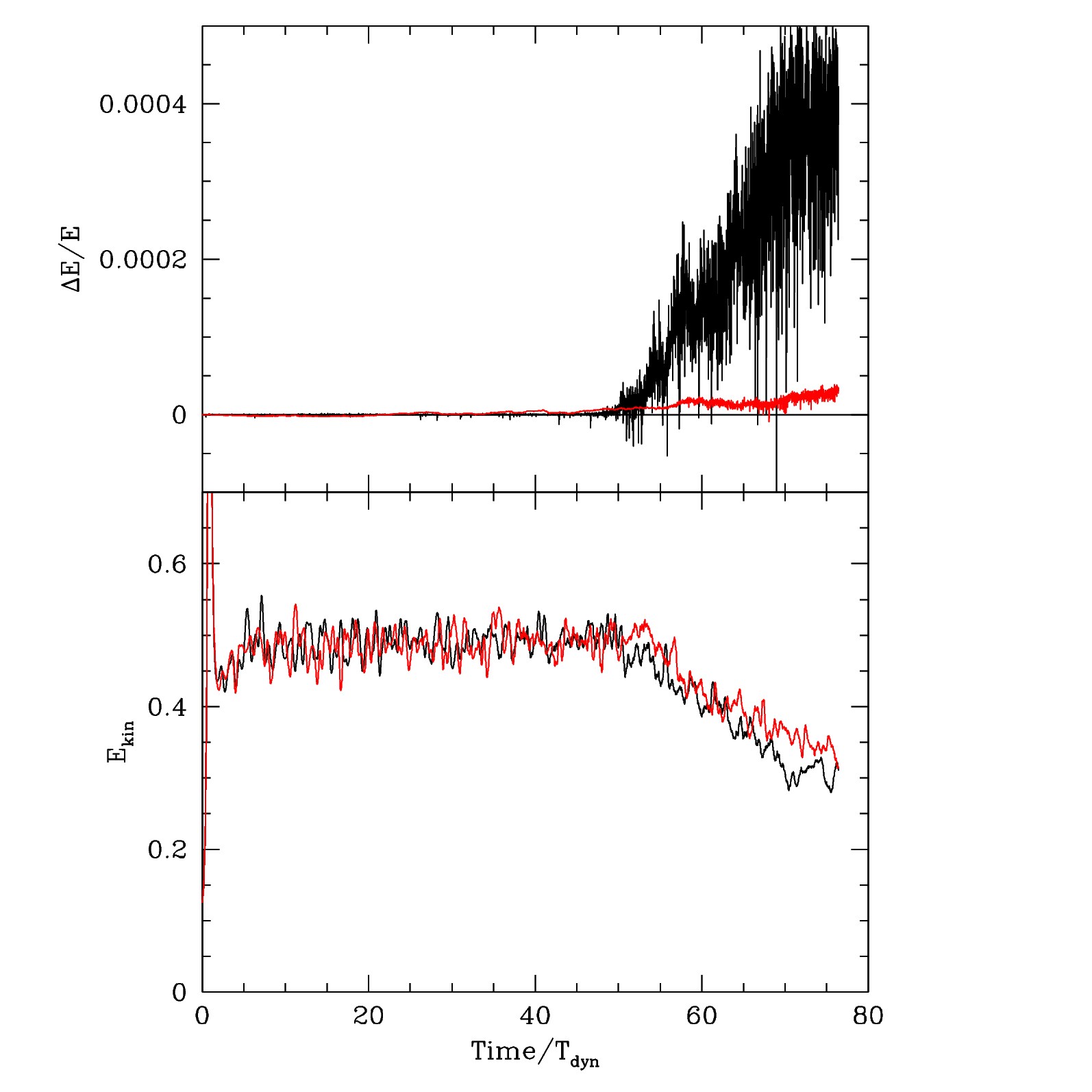
The real advantage of the variable step is in the reduced drift of the direction of the main axis. The bottom panel shows every 100th orbit. The last one is the 1000th orbit. If you compare this with the first plot, where only the 1000th orbit is shown, it is clear that the variable time step improves the accuracy dramatically.

Simulations with constant time-step: dt=3.2e-3. Number of force estimates per orbit is 1500. The energy conservation plot shows dE/E averaged over three output moments. There are 15 output moments per orbit. The averaging reduces the maximum error by a factor three. The maximum error occurs at the moment of smallest radius. It does not propagate in time.

Evolution of a system of 500 equal-mass objects. Here we compare two runs: one with constant step (black curves) and another with a variable step (red curves). Both runs have the same number of force evaluations.
Initial distribution is a homogeneous sphere with unit radius and with the ratio of kinetic to potential energy equal to Ekin/Epot=0.2. As the system shrinks, its kinetic energy increases. It reaches value Ekin=1.2 at t=1.2. Then the system gets to virial equilibrium. As time goes on, collisions between individual particles result in formation of binaries. At the end of the run there were about 10 binaries.

Constant step leapfrog was not able to integrate the binaries (and the scatter of other particles) accurately enough. So, energy conservation started to degrade. Variable time-stepping is lot better because it does not loose the energy as much as the constant step scheme.

Force softening is equal to 0.001. Initial radius is 1. Initial 1d rms velocities are 0.2755. Dynamical time is pi/2.
Constant step: dt= 5.4e-5. Number of force evaluations is 2.9e4 per particle per dynamical time.
Variable step: large step dt=2e-4, number of refinement levels 4 (max decrease in step is 16). aStep=3e-3 (displacement of coordinates), Alph=5e-4 (relative change in velocity).

Evolution of a system of 5000 equal-mass objects. The force softening is 1.e-4 . This is ten times smaller than for the previous plot. Run with constant step is shown by blue curves; a variable step is red curves. The constant times step was doing really badly. It had 3 times more gravity evaluations and yet its error was 100 times larger already during the first 10 dynamical times.

Force softening is equal to 0.0001. Initial radius is 1. Initial 1d rms velocities are 0.2755. Dynamical time is pi/2.
Constant step: dt= 5.4e-5. Number of force evaluations is 2.9e4 per particle per dynamical time.
Variable step: large step dt=4e-4, number of refinement levels 5 (max decrease in step is 32), aStep=2e-3 (displacement of coordinates), Alph=1e-3 (relative change in velocity). Number of force evelutions 1.e4 per particle per dynamical time